[Problem Set 4 Networks] Problem 2: Circuit with mutual inhibition
Link of the iPython notebook for the code
AT2 – Neuromodeling: Problem set #4 NETWORKS
PROBLEM 2: Circuit with mutual inhibition
Now, let us consider a two-neurons circuit in which the neurons mutually inhibit one another. We will denote by
- $x_1$ and $x_2$ the firing rates of the two neurons
- $w = -0.1$ the inhibitory synaptic weight
- $I = 5$ an excitatory external input
- $f(s) ≝ 50 \, (1 + \tanh(s))$ the neurons’ activation function as before
1. Separate treatement of each neuron
We assume that we have the following differential equations:
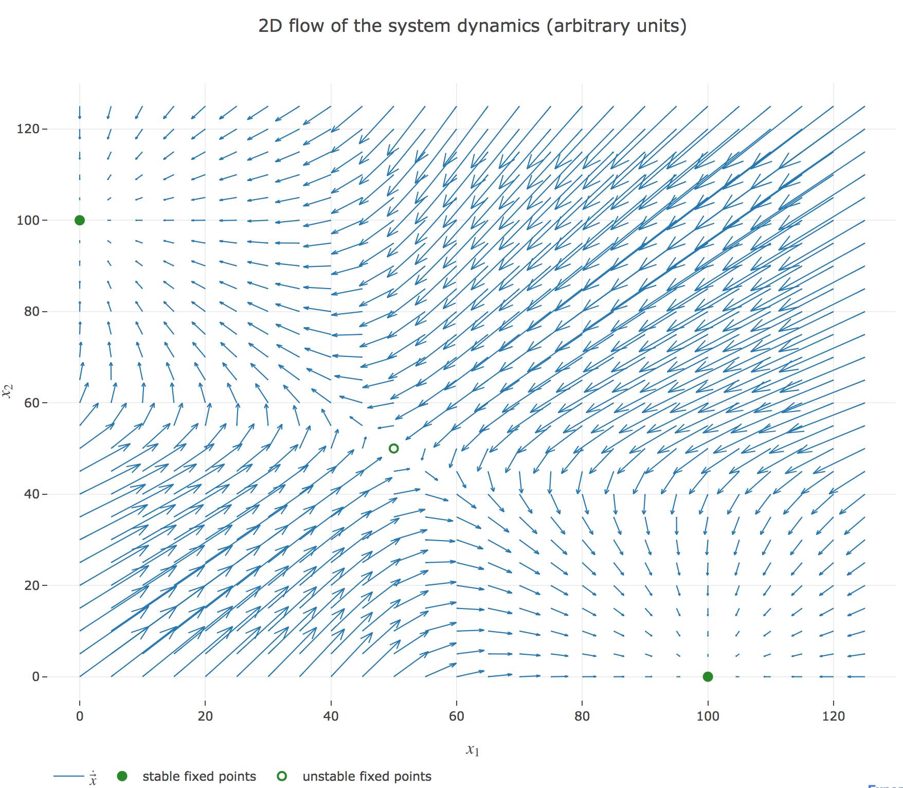
\[\begin{cases} \dot{x}_1(t) = -x_1(t) + f(w x_2(t) + I)\\ \dot{x}_2(t) = -x_2(t) + f(w x_1(t) + I)\\ \end{cases}\]which results in the following two-dimensional system dynamics flow:
The nullclines of this system are the curves given by:
\[\begin{cases} \dot{x}_1(t) = 0 \\ \dot{x}_2(t) = 0 \end{cases}\]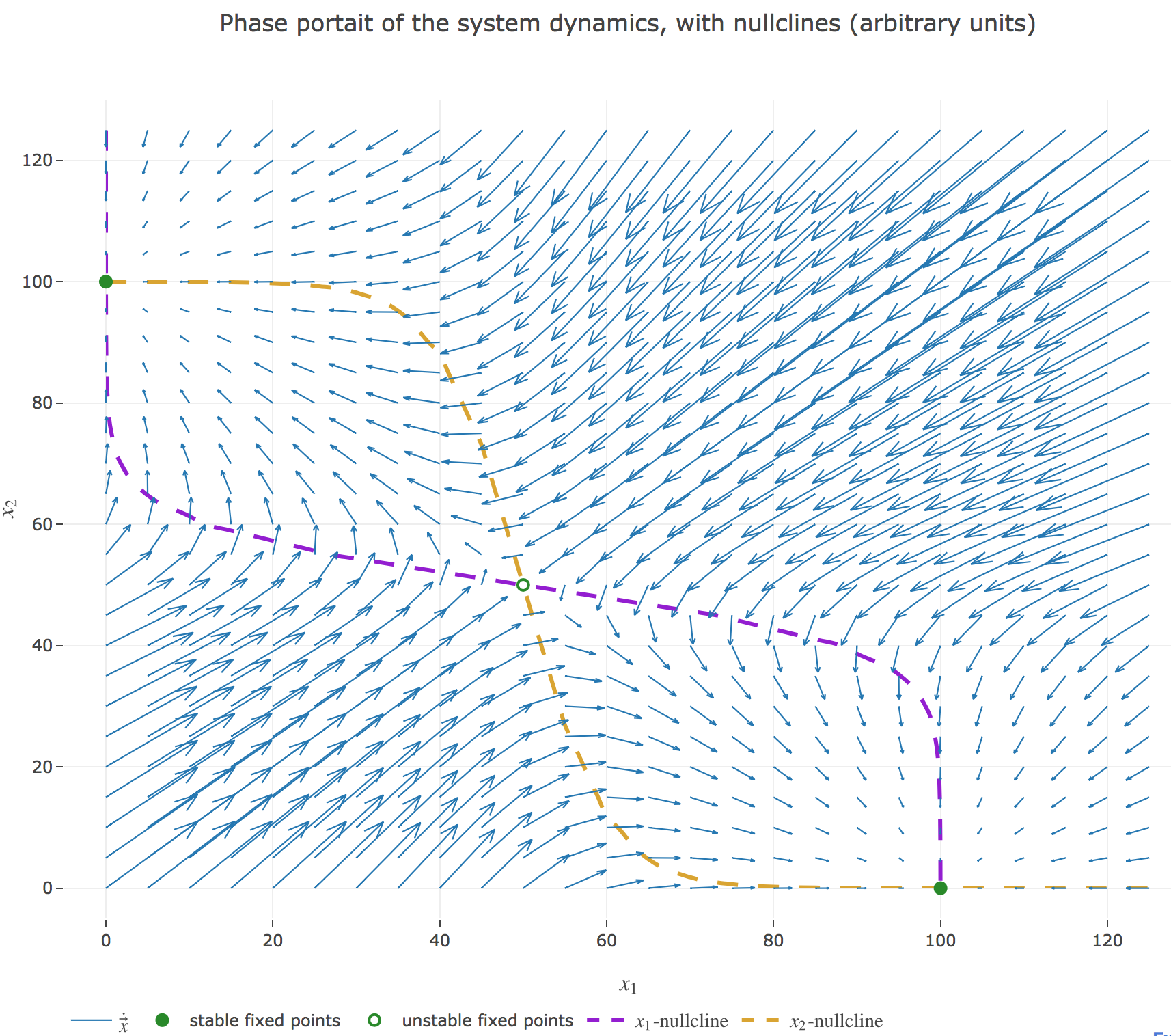
Their crossing points are the points at which both the $x_1$ derivative and the $x_2$ one vanish, i.e. the fixed points of the 2D-system dynamics. As before (cf. the previous problem), there are:
- stable fixed points: here, the points $(0, 100)$ and $(100, 0)$
- unstable fixed points: here, the point $(50, 50)$
We can easily check these are indeed fixed points of the dynamics:
-
For $(0, 100)$:
\[\begin{align*} -0+f(100w + I) &= f(-5) = 50(1+\tanh(-5))≃ 0 \\ -100+f(0w + I) &= f(5)-100 = 50(\underbrace{1+\tanh(5)}_{≃ 2}) - 100 ≃ 0 \end{align*}\]and it is symmetric for $(100, 0)$
-
For $(50, 50)$:
\[\begin{align*} -50+f(50w + I) &= f(0) - 50 = 50(1+\underbrace{\tanh(0)}_{=0}) - 50 = 0 \\ \end{align*}\]
System simulation
We set (arbitrary units):
- the time-increment to integrate the differential equation with the Euler method: $dt = Δt ≝ 0.1$
- The total duration $T = 10 = 100 Δt$
so that the Euler method yields, for $i ≠ j ∈ \lbrace 1, 2 \rbrace$:
\[\begin{align*} \quad & \frac{x_i(t+Δt) - x_i(t)}{Δt} = - x_i(t) + f\big(wx_j(t) + I\big) \\ ⟺ \quad & x_i(t+Δt) - x_i(t) = - x_i(t) Δt + f\big(wx_j(t) + I\big) Δt \\ ⟺ \quad & x_i(t+Δt) = (1 - Δt) x_i(t) + f\big(wx_j(t) + I\big) Δt \end{align*}\]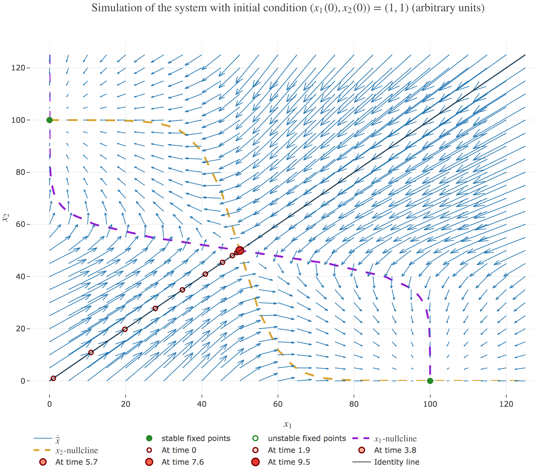
It appears that:
-
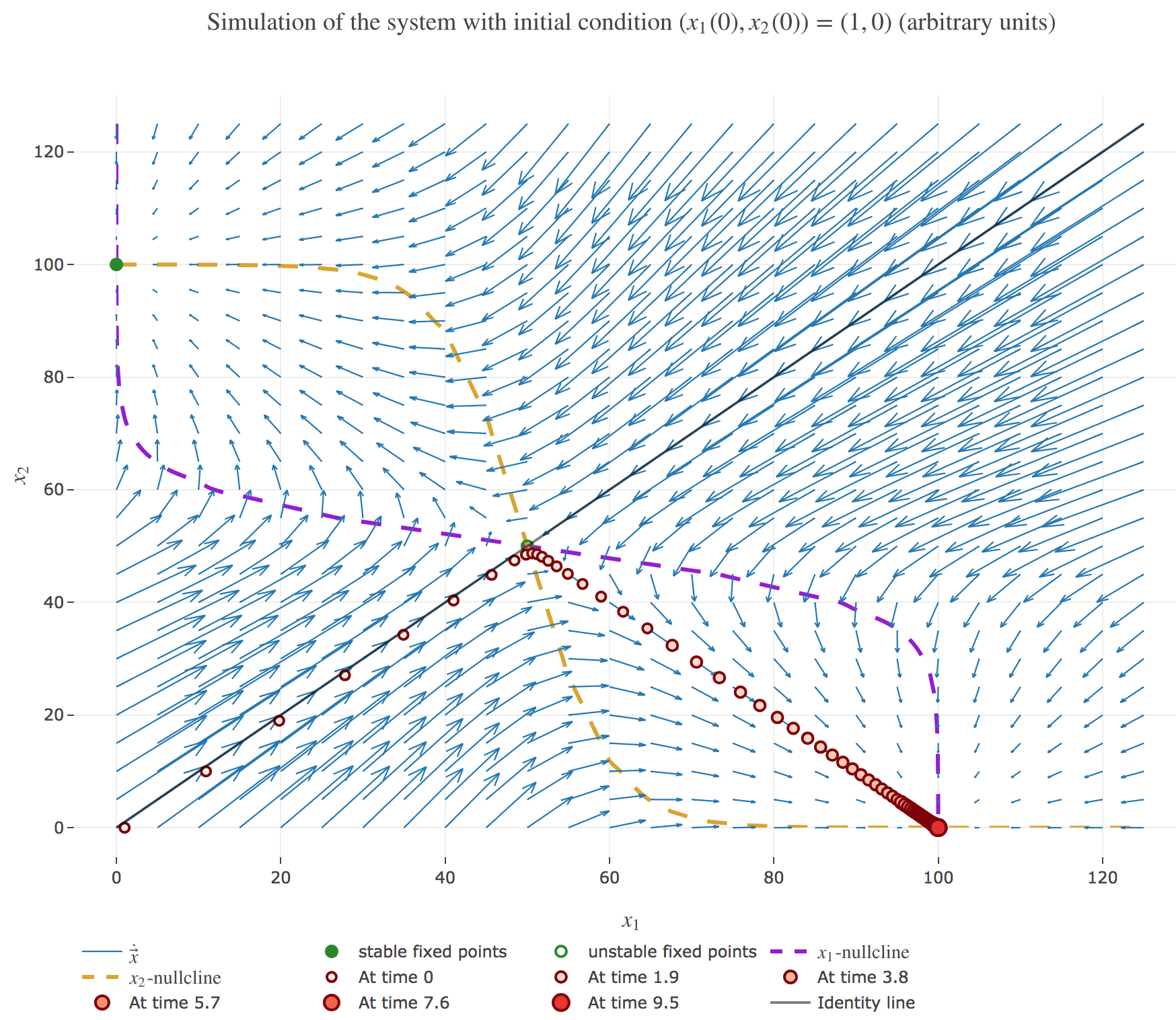
if $(x_1(0), x_2(0))$ is on the identity line – i.e. if $x_1(0) = x_2(0)$) – : $(x_1(t), x_2(t))$ converges toward the $(50, 50)$ unstable fixed point, as exemplified by figure 1.b.1.
-
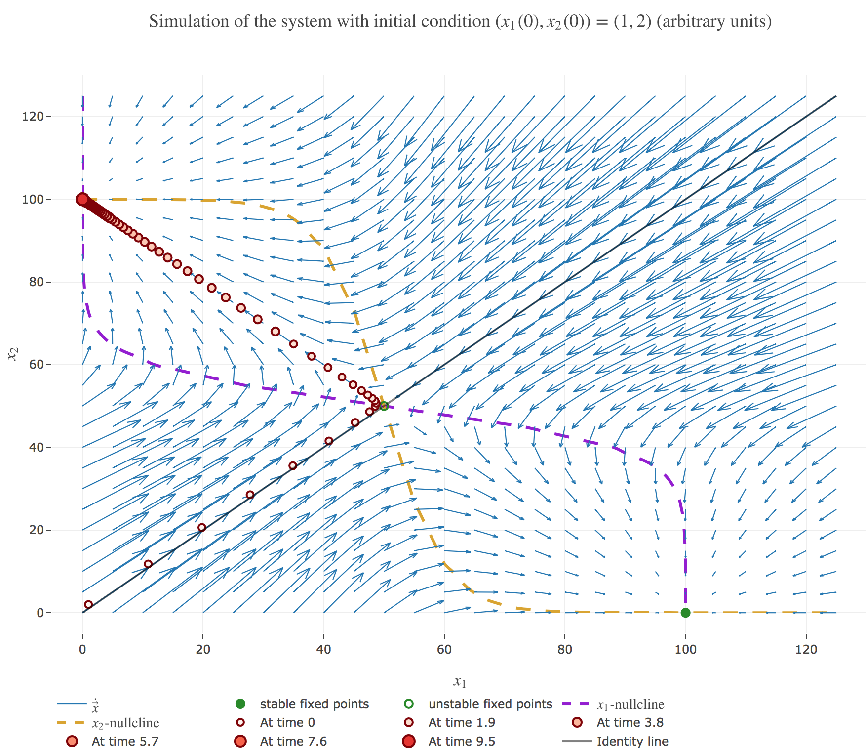
if $(x_1(0), x_2(0))$ is strictly above the identity line – i.e. if $x_1(0) < x_2(0)$) – : $(x_1(t), x_2(t))$ converges toward the $(0, 100)$ stable fixed point, as exemplified by figure 1.b.2.
-
if $(x_1(0), x_2(0))$ is strictly below the identity line – i.e. if $x_1(0) > x_2(0)$) – : $(x_1(t), x_2(t))$ converges toward the $(100, 0)$ stable fixed point, as exemplified by figure 1.b.3.
2. Vectorized system dynamics
We have hitherto treated each neuron separately, but there is a way to reduce the two differential equations to a single vectorized one:
\[\dot{\textbf{x}}(t) = - \textbf{x}(t) + f(W \textbf{x}(t) + \textbf{I})\]by setting:
- \[\textbf{x}(t) ≝ \begin{pmatrix} x_1(t)\\ x_2(t)\end{pmatrix} ∈ 𝔐_{2,1}(ℝ)\]
- \[W ≝ \begin{pmatrix} 0 & w\\ w & 0\end{pmatrix} ∈ 𝔐_2(ℝ)\]
- \[I ≝ \begin{pmatrix} I\\ I\end{pmatrix} ∈ 𝔐_{2,1}(ℝ)\]
as a result of which the Euler method gives:
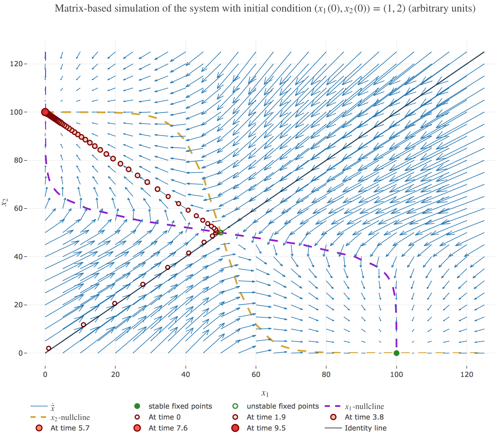
\[\begin{align*} \quad & \frac 1 {Δt}\Big(\textbf{x}(t+Δt) - \textbf{x}(t)\Big) = - \textbf{x}(t) + f(W \textbf{x}(t) + \textbf{I}) \\ ⟺ \quad & \textbf{x}(t+Δt) = (1 - Δt)\, \textbf{x}(t) + Δt \, f(W \textbf{x}(t) + \textbf{I}) \end{align*}\]And we get the same simulations as before, for example with the initial condition $(x_1(0), x_2(0)) ≝ (1, 2)$:
Leave a comment