[Problem Set 4 Networks] Problem 1: Neuron with Autapse
Link of the iPython notebook for the code
AT2 – Neuromodeling: Problem set #4 NETWORKS
PROBLEM 1: Neuron with Autapse
1. One-dimensional deterministic dynamical system
Let us consider a neuron whose axons connects to its own dendrites (the resulting synapse is called an autapse): we will denote by
- $x$ its firing rate
- $w = 0.04$ the strength of the synaptic connection
- $I = -2$ an external inhibitory input
-
$f(s) ≝ 50 \, (1 + \tanh(s))$ the neuron’s activation function, where $s$ is the overall neuron input:
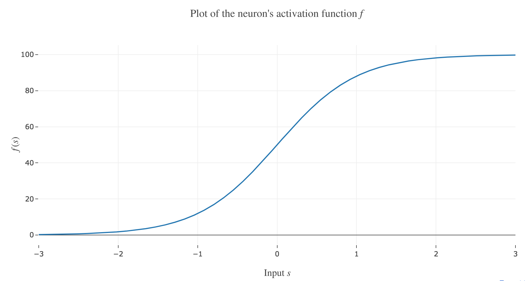
Figure 1.a. - Plot of the neuron's activation function $f$
(in arbitrary units) so that the firing rate is described by the following differential equation:
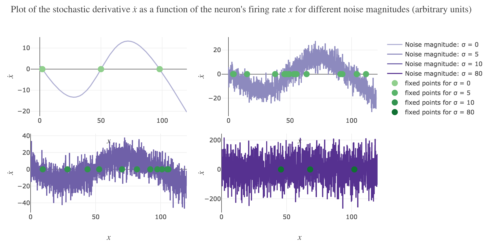
\[\dot{x}(t) = - x(t) + f\big(wx(t) + I\big)\]Plotting the derivative $\dot{x}$ as a function of the neuron’s firing rate $x$:
\[x ⟼ - x + f\big(wx + I\big)\]results in the following 1-dimensional system dynamics:
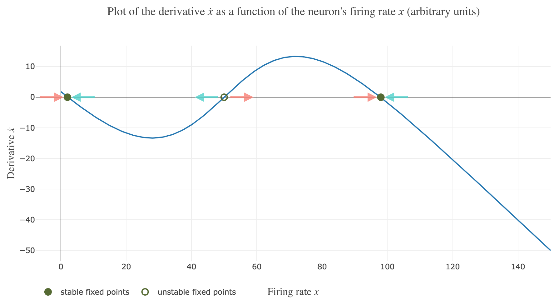
The zero-crossings of $\dot{x}$ as a function of $x$ correspond to critical points, i.e. values of $x$ at which the derivative $t ⟼ \dot{x}(t)$ equals zero, hence the function $t ⟼ x(t)$ being constant with respect to $t$. As a consequence, such values of $x$ at which $\dot{x}$ (as a function of $x$) vanishes are called fixed point of the dynamics, as $x$ is left unchanged over time.
Dynamics fixed points are twofold:
-
stable fixed points (attractors) are fixed points around which a slight change of $x$ leads to $x$ moving back to the stable fixed point value: these correspond to points $x^\ast$ such that the derivative $\dot{x}$ is:
- positive at $x^\ast-ε$ ($x$ increases back to $x^\ast$)
- negative at $x^\ast+ε$ ($x$ decreases back to $x^\ast$)
for $ε>0$ sufficiently small. In other words, the zero-crossing goes from positive values to negative ones.
On Figure 1.b., the two stable fixed points at $x=2$ and $x=98$ are indicated by a filled up green point.
-
unstable fixed points (repellers) are fixed points around which a slight change of $x$ leads to $x$ moving away from the unstable fixed point value: these correspond to points $x^\ast$ such that the derivative $\dot{x}$ is:
- negative at $x^\ast-ε$ ($x$ keeps decreasing away from $x^\ast$)
- positive at $x^\ast+ε$ ($x$ keeps increasing away from $x^\ast$)
for $ε>0$ sufficiently small. In other words, the zero-crossing goes from negative values to positive ones.
On Figure 1.b., the only unstable fixed point at $x=50$ is indicated by a hollow green circle.
Now, let us simulate the system for various initial conditions:
\[x(0) ∈ \Big\lbrace \overbrace{49}^{\llap{\text{just below the unstable fixed point}}}\,, \underbrace{50}_{\text{the unstable fixed point}}, \overbrace{51}^{\rlap{\text{just above the unstable fixed point}}} \Big\rbrace\]We set (arbitrary units):
- the time-increment to integrate the differential equation with the Euler method: $dt = Δt ≝ 0.1$
- The total duration $T = 10 = 100 Δt$
so that the Euler method yields:
\[\begin{align*} \quad & \frac{x(t+Δt) - x(t)}{Δt} = - x(t) + f\big(wx(t) + I\big) \\ ⟺ \quad & x(t+Δt) - x(t) = - x(t) Δt + f\big(wx(t) + I\big) Δt \\ ⟺ \quad & x(t+Δt) = (1 - Δt) x(t) + f\big(wx(t) + I\big) Δt \end{align*}\]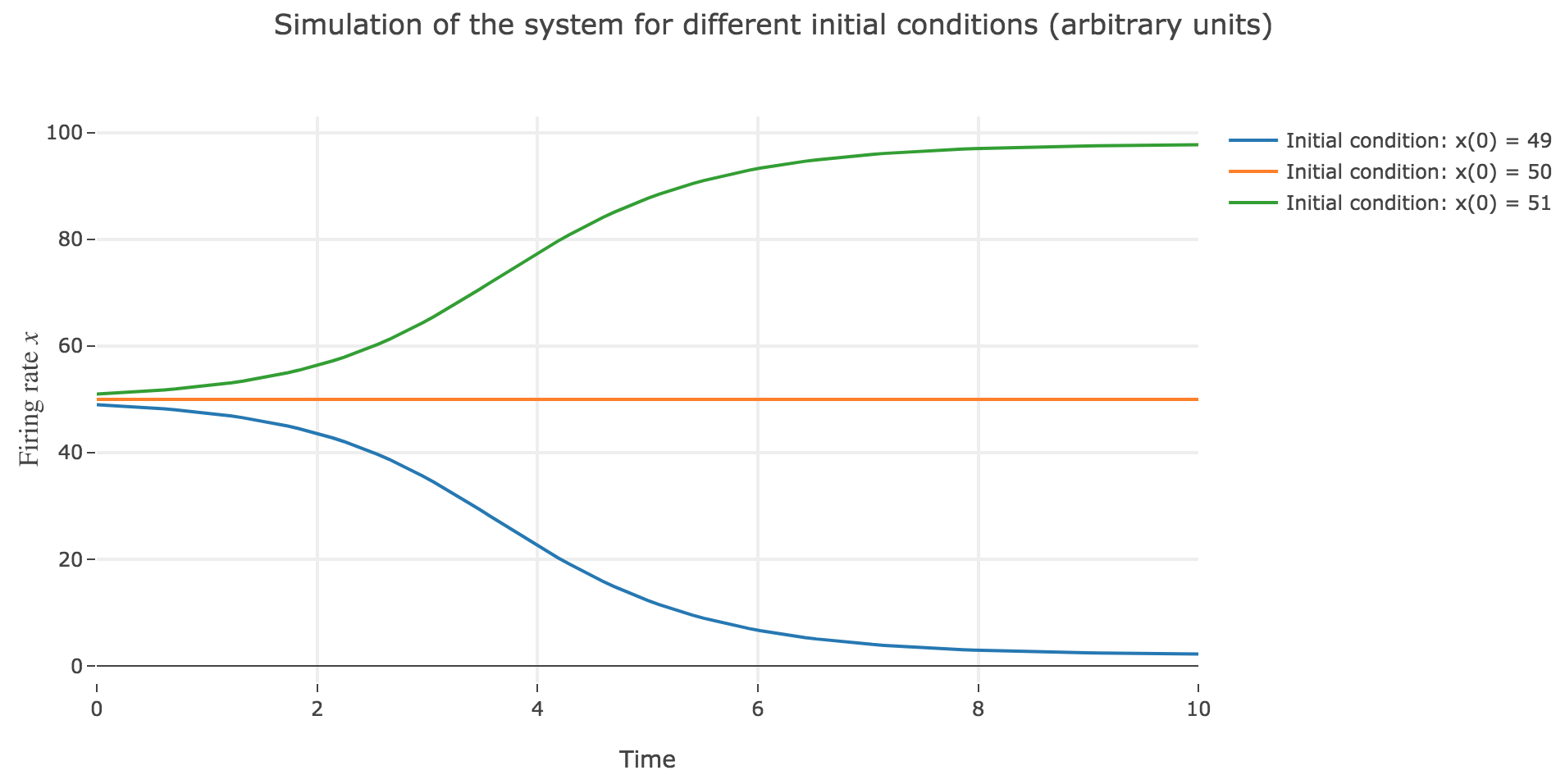
As expected, since $x=50$ is an unstable fixed point of the dynamics: when
-
$x(0) = 50$: $x(t)$ remains constantly equal to $50$ over time (as $50$ is a fixed point)
-
$x(0) = 51 > 50$: $x(t)$ keeps increasing, converging to the (stable) fixed point $98$, since the time derivative $\dot{x}$ is strictly positive at $98 > x >50$ (cf. Figure 1.b.)
-
$x(0) = 49 < 50$: $x(t)$ keeps decreasing, converging to the (stable) fixed point $2$, since the time derivative $\dot{x}$ is strictly negative at $2 < x<50$ (cf. Figure 1.b.)
2. One-dimensional stochastic dynamical system
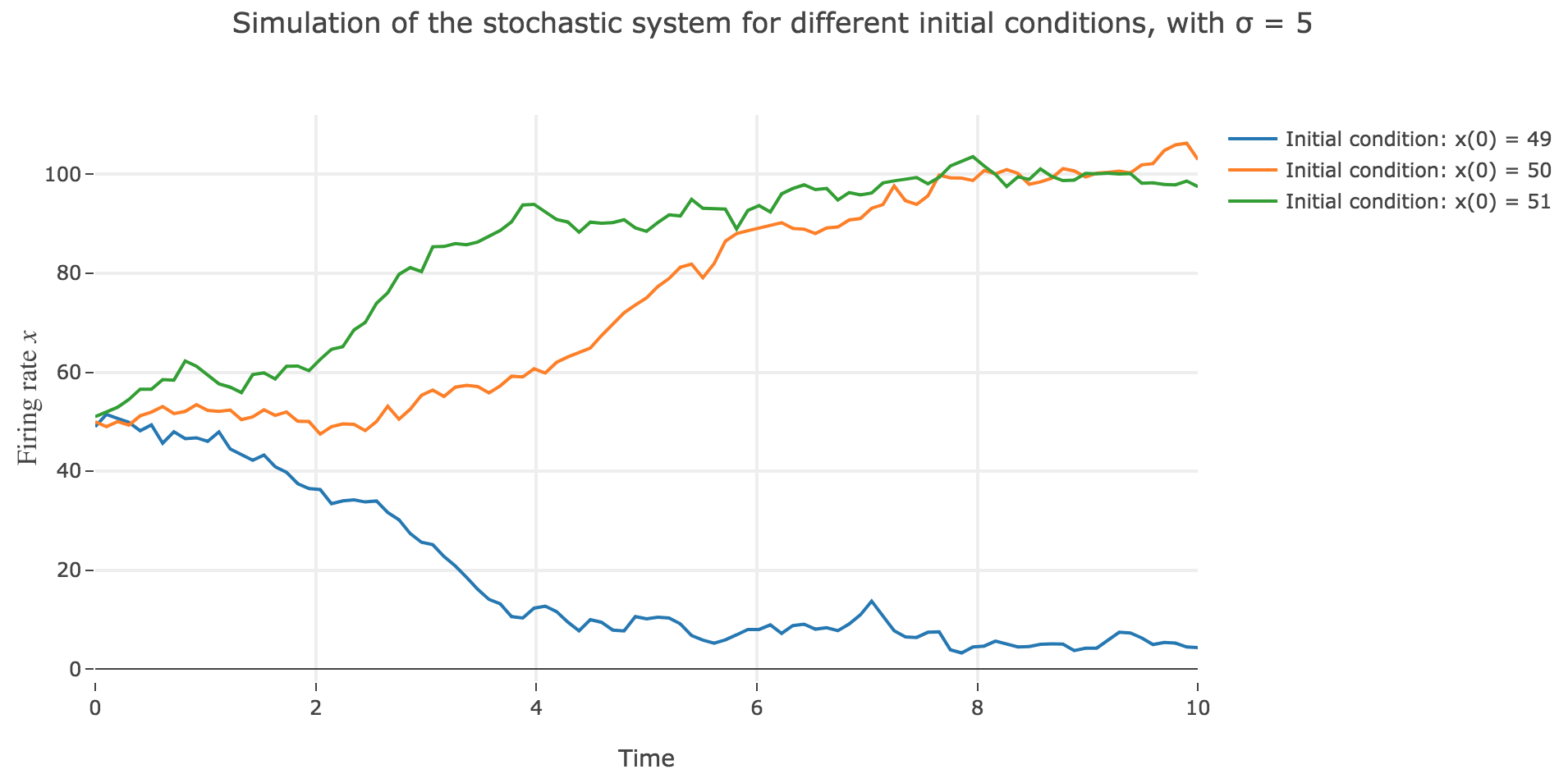
From now on, for the sake of realism, we add a white noise component to the system:
\[\dot{x}(t) = - x(t) + f\big(wx(t) + I\big) + σ η(t)\]where $η(t)$ is a Gaussian noise, $σ$ is the noise magnitude.
The stochastic differential equation is solved numerically as follows:
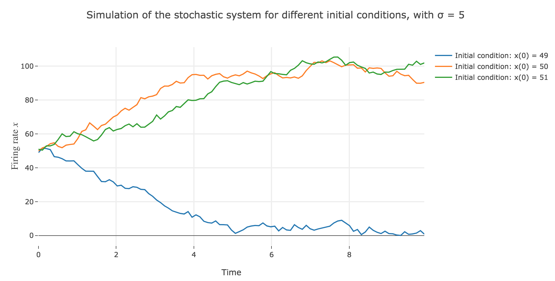
\[\begin{align*} \quad & x(t+Δt) - x(t) = - x(t) Δt + f\big(wx(t) + I\big) Δt + σ η(t) \sqrt{Δt} \\ ⟺ \quad & x(t+Δt) = (1 - Δt) x(t) + f\big(wx(t) + I\big) Δt + σ η(t) \sqrt{Δt} \end{align*}\]which leads to (for $σ = 5$ and several random seeds):
-
the $x(0)=50$ initial condition starts from an unstable fixed point of the dynamics (as seen before) when there is no noise: any slight variation of $x$ relative to this unstable fixed point leads to $x(t)$ moving away from this value. As it happens, here, this variation stems from the noise added to the time derivative $\dot{x}$, which results in the unstable fixed point being slighly moved aside, leading to $x(t)$ ending up above or below this unstable fixed point, and thus converging toward one the two stable fixed points ($2$ and $98$), depending on whether the noise variation has drawn the unstable fixed point:
- above $x$ (leading $x$ to decrease toward $2$), as in figure 2.d.1.3
- or below $x$ (leading $x$ to increase toward $98$), as in figures 2.d.1.1 and 2.d.1.2
-
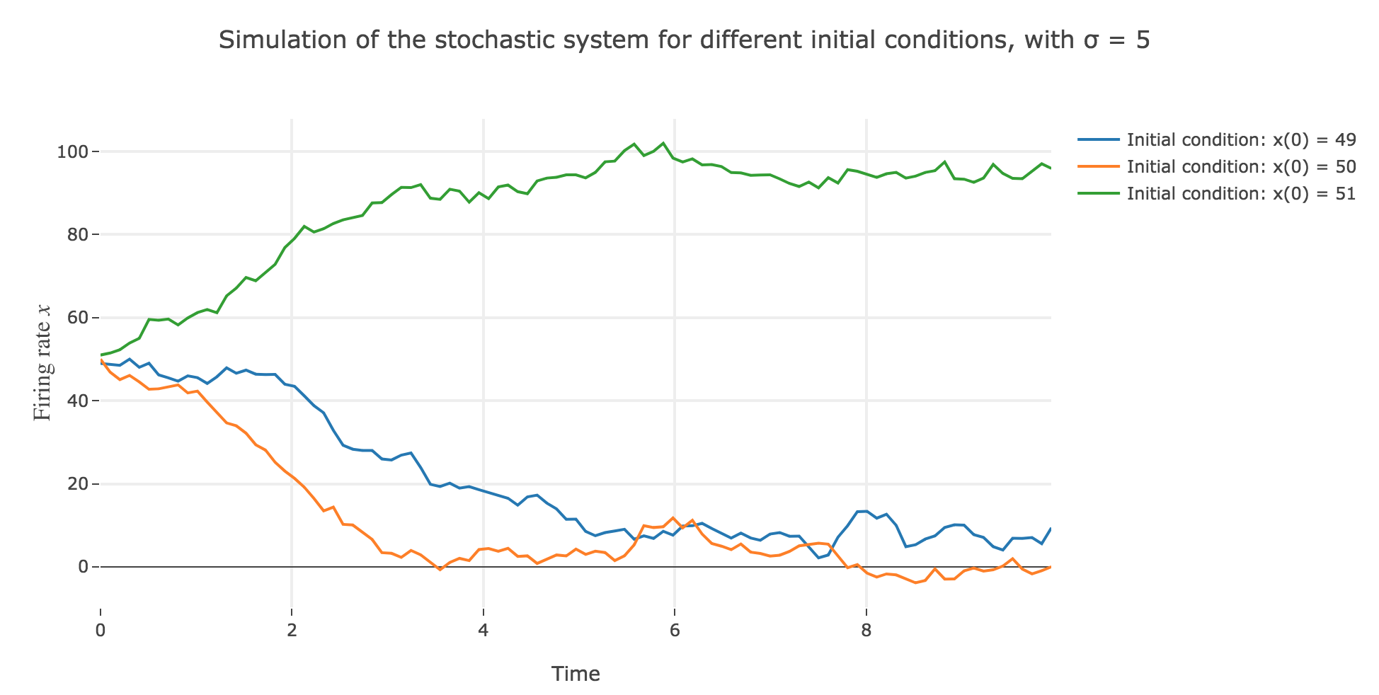
the $x(0) = 49$ (resp. $x(0) = 51$) initial conditions causes $x(t)$ to decrease (resp. increase) toward the stable fixed point $2$ (resp. $98$) when there is no noise (as seen before): any slight variation of $x$ relative to these stable fixed points bring $x(t)$ back to them. The only possibility for $x$ not to converge toward $2$ (resp. $98$) instead would be that the noise added to derivative has such a magnitude that it makes it positive (resp. negative) at $x$, which doesn’t happen in the three figures 2.d.1.1, 2.d.1.2, and *2.d.1.3**: the added noise magnitude is too small: $x$ still converges toward the expected fixed point.
Now for various noise magnitudes:
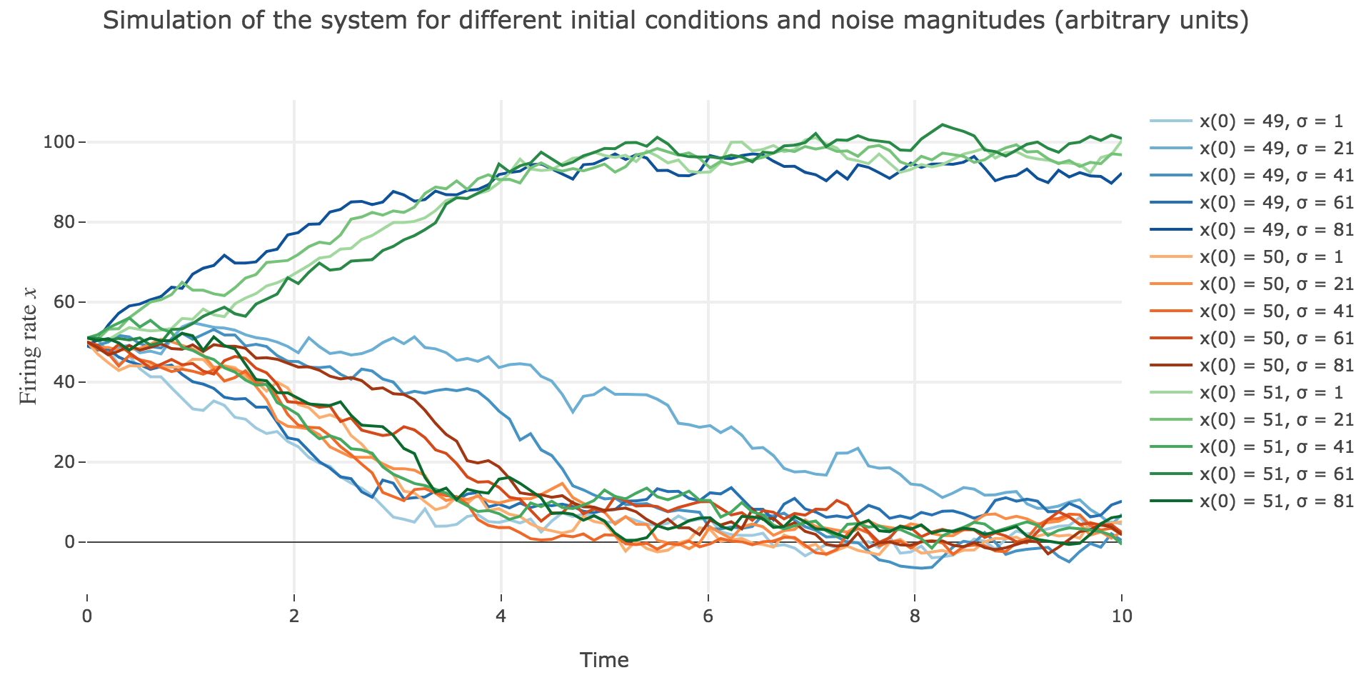
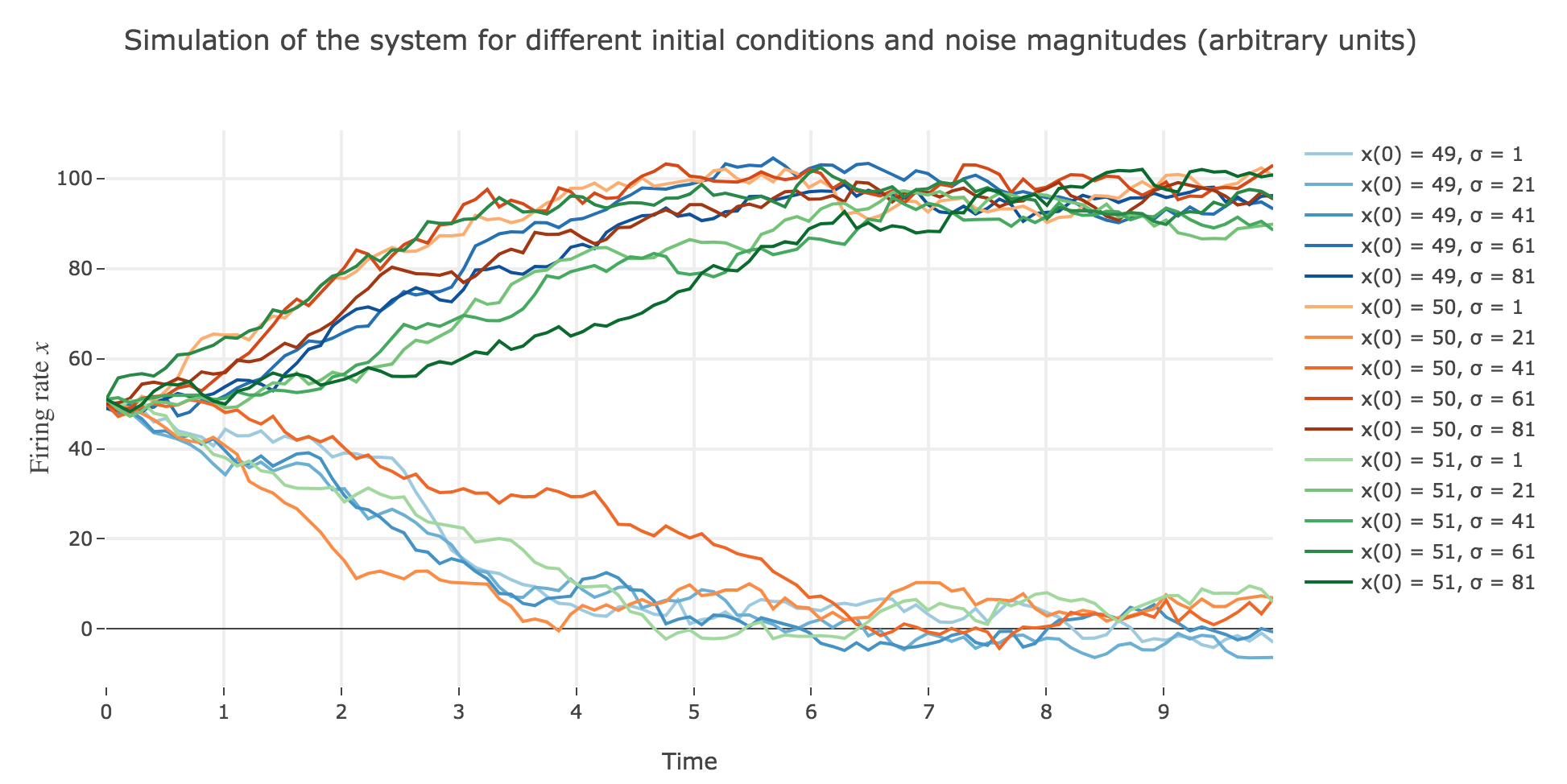
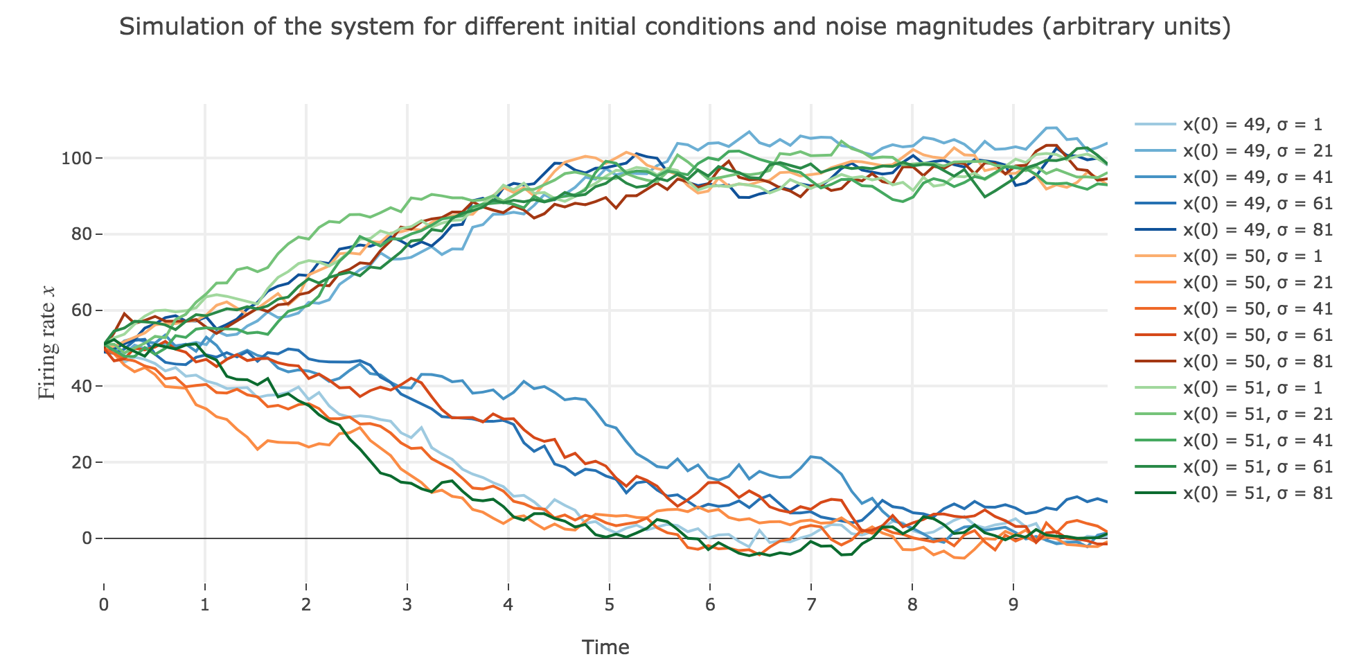
As the initial condition $x(0)=50$ starts from an unstable fixed point of the deterministic dynamics, $x$ may equiprobably converge to one the two stable fixed points when adding the noise, which makes this case of little interest (it clutters the graphs uselessly). We may as well only plot the remaining relevant cases ($x(0) ∈ \lbrace 49, 51 \rbrace$):
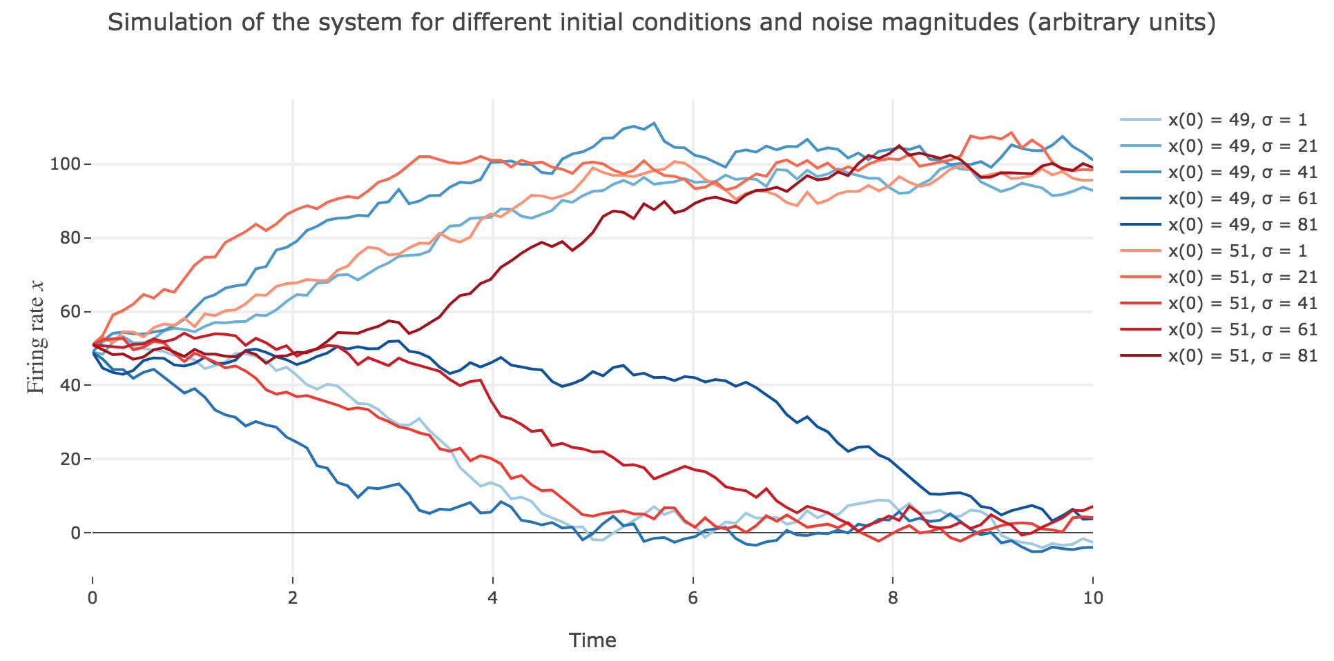
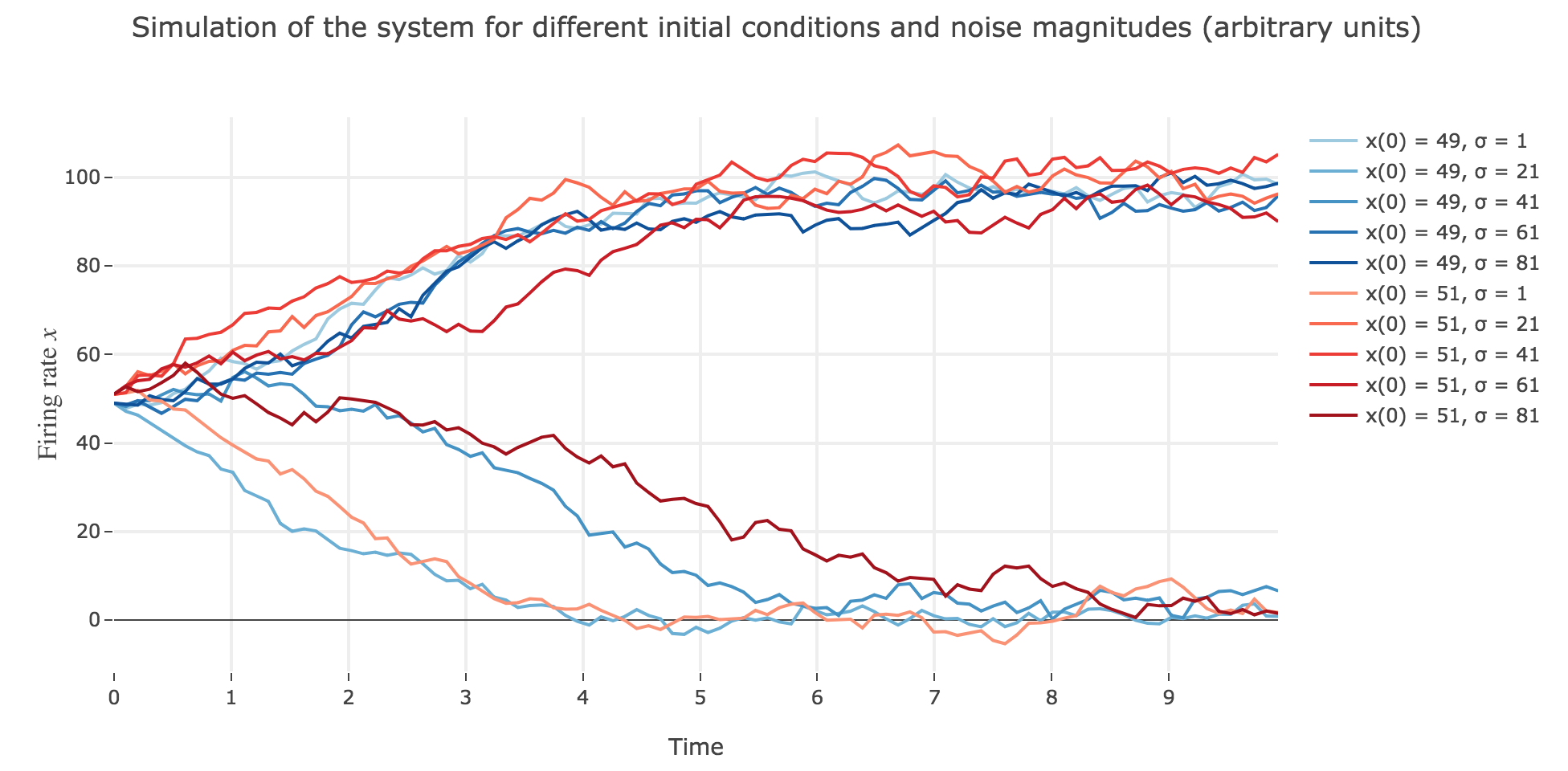
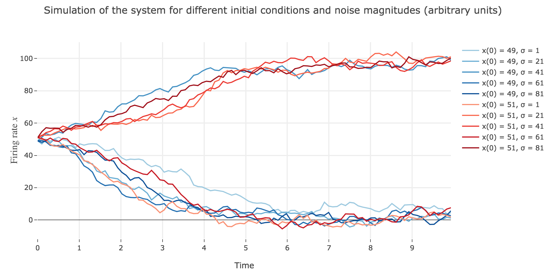
What appears in the above figures is that the bigger the noise magnitude $σ$ is, the more $x(t)$ is likely not to converge toward the expected stable fixed point (i.e. $98$ for $x>50$, $2$ for $x<50$).
This can be accounted for by the fact that the fixed points of dynamics change all the more that the noise magnitude is larger and larger: indeed, the larger the noise magnitude, the more the derivative $\dot{x}$ is modified (as the noise is added to it) and the more it moves away from its original value: new zero-crossings (i.e. fixed points) appear, other disappear, etc…:
To back this up: here is the evolution of the fixed points of the dynamics for different noise magnitudes (and different random seeds):
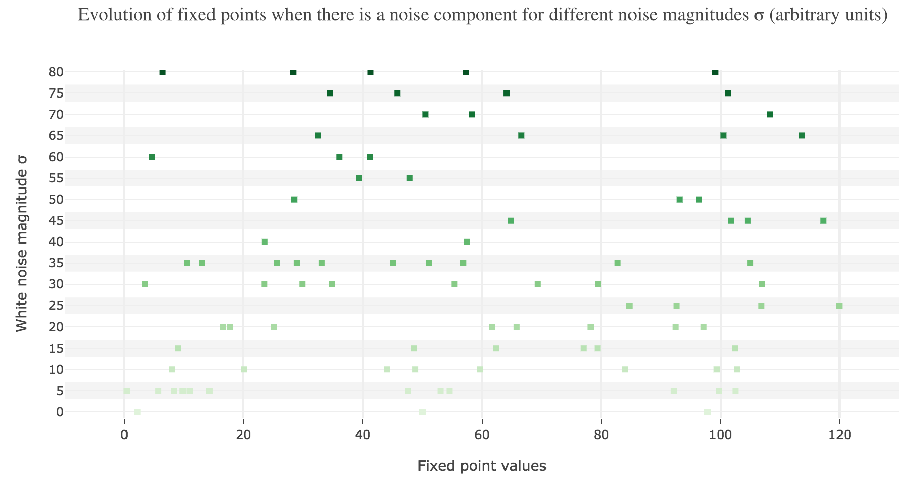
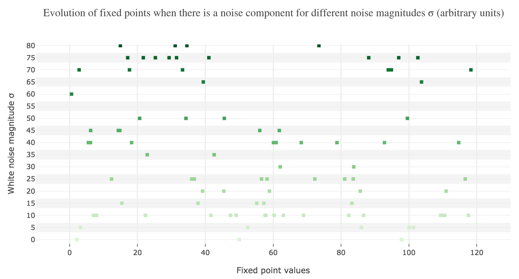
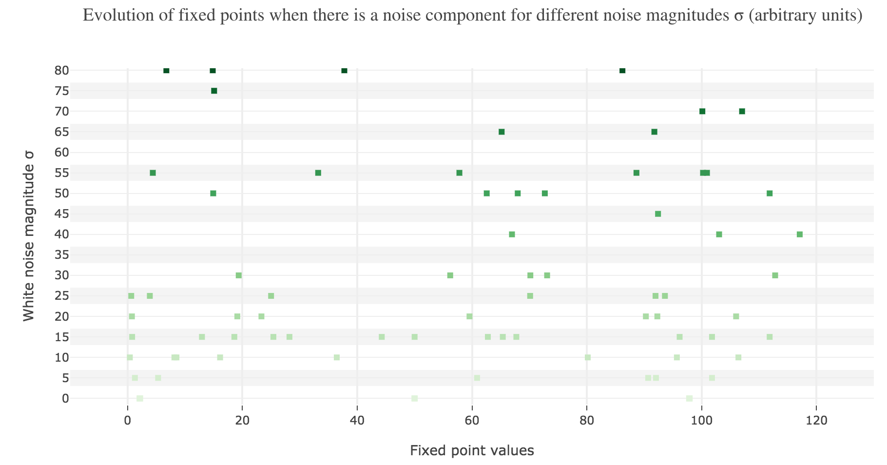
So the larger the noise magnitude, the “more” the set of fixed points is modified, resulting in $x(t)$ being less and less likely to converge toward the expected stable fixed point ($98$ for $x>50$, $2$ for $x<50$).
Leave a comment