[Problem Set 4 Networks] Problem 3: Hopfield model
Link of the iPython notebook for the code
AT2 – Neuromodeling: Problem set #4 NETWORKS
PROBLEM 3: Hopfield Model
\[\newcommand{\T}{ {\raise{0.7ex}{\intercal}}} \newcommand{\sign}{\textrm{sign}}\]We will study the properties of a Hopfield network with $N = 64$ neurons, whose dynamics obeys the following differential equation:
\[\dot{\textbf{x}} = - \textbf{x} + f(W \textbf{x}) + σ η(t)\]where
-
$\textbf{x}$ is the firing rates vector
-
$W$ is the $N × N$ weight matrix
-
$η(t)$ is a Gaussian noise of magnitude $σ = 0.1$
-
the activation function $f ≝ \sign$ for the sake of simplicity
1. Storing a pattern
A pattern $\textbf{p} ∈ 𝔐_{N,1}(\lbrace -1, 1 \rbrace)$ is stored in the Hopfield network by setting:
\[W ≝ \frac 1 N \textbf{p} \textbf{p}^\T\]Here are some examples of patterns, visualized as $8×8$ images:
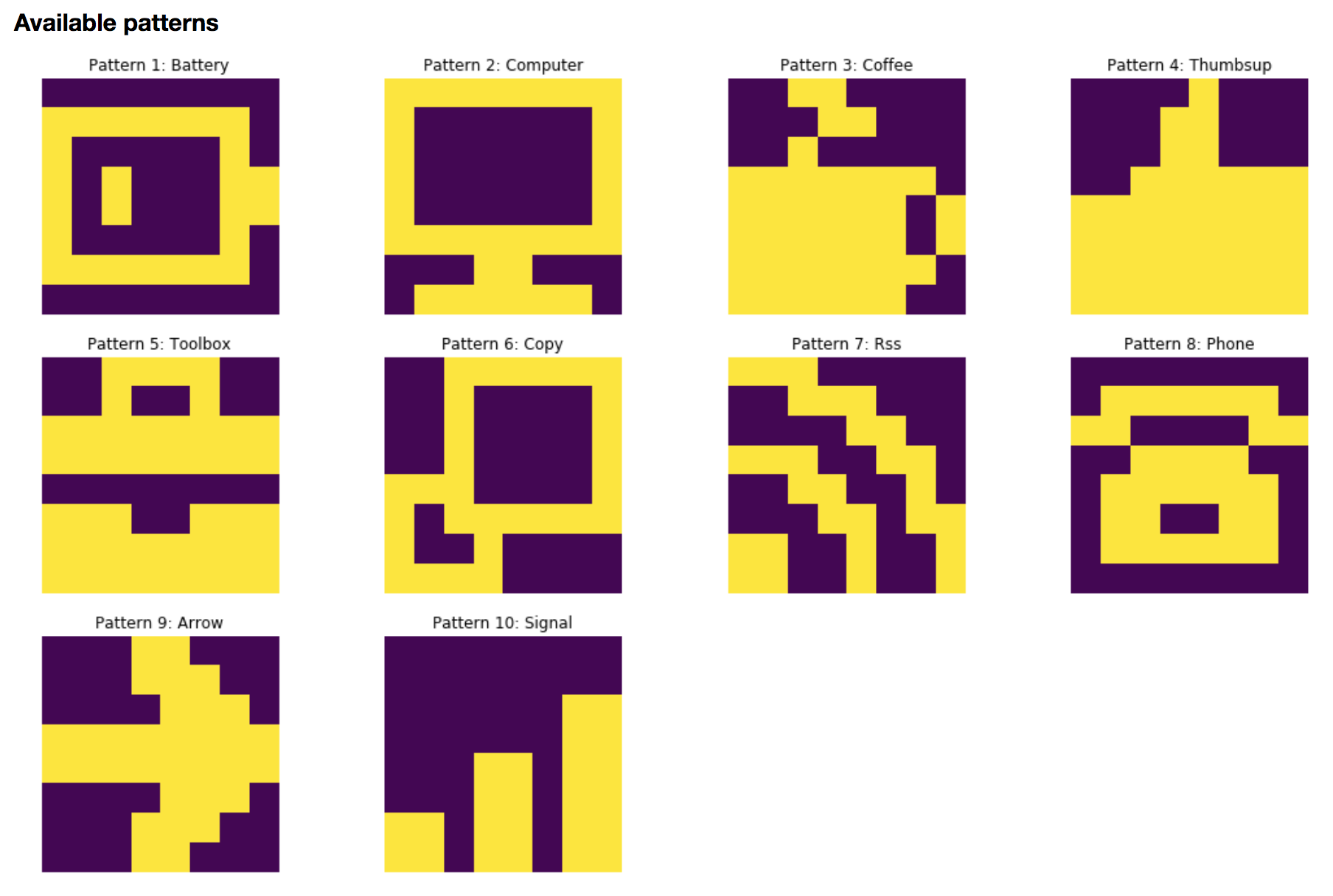
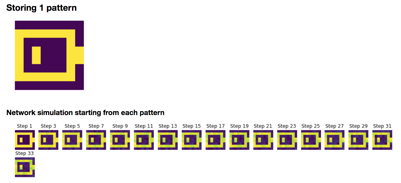
To begin with, let us focus on storing the battery pattern $\textbf{p}_{\text{bat}}$:
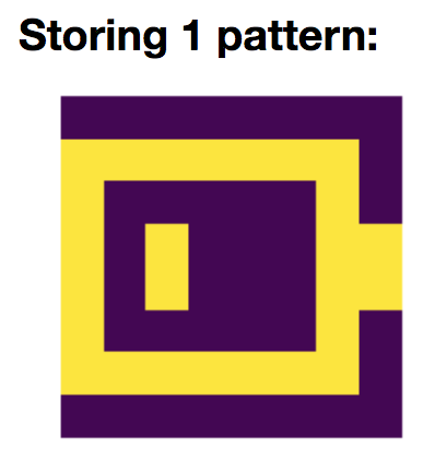
We set
\[W ≝ \frac 1 N \, \textbf{p}_{\text{bat}} \textbf{p}^\T_{\text{bat}}\]Then, we simulate the network with resort to the Euler method (with time-increment $dt = Δt ≝ 0.1$ (arbitrary units)):
\[\textbf{x}(t+Δt) = (1 - Δt)\, \textbf{x}(t) + Δt \, \sign(W \textbf{x}(t)) + \sqrt{Δt} \, σ η(t)\]which yields, for random starting patterns:
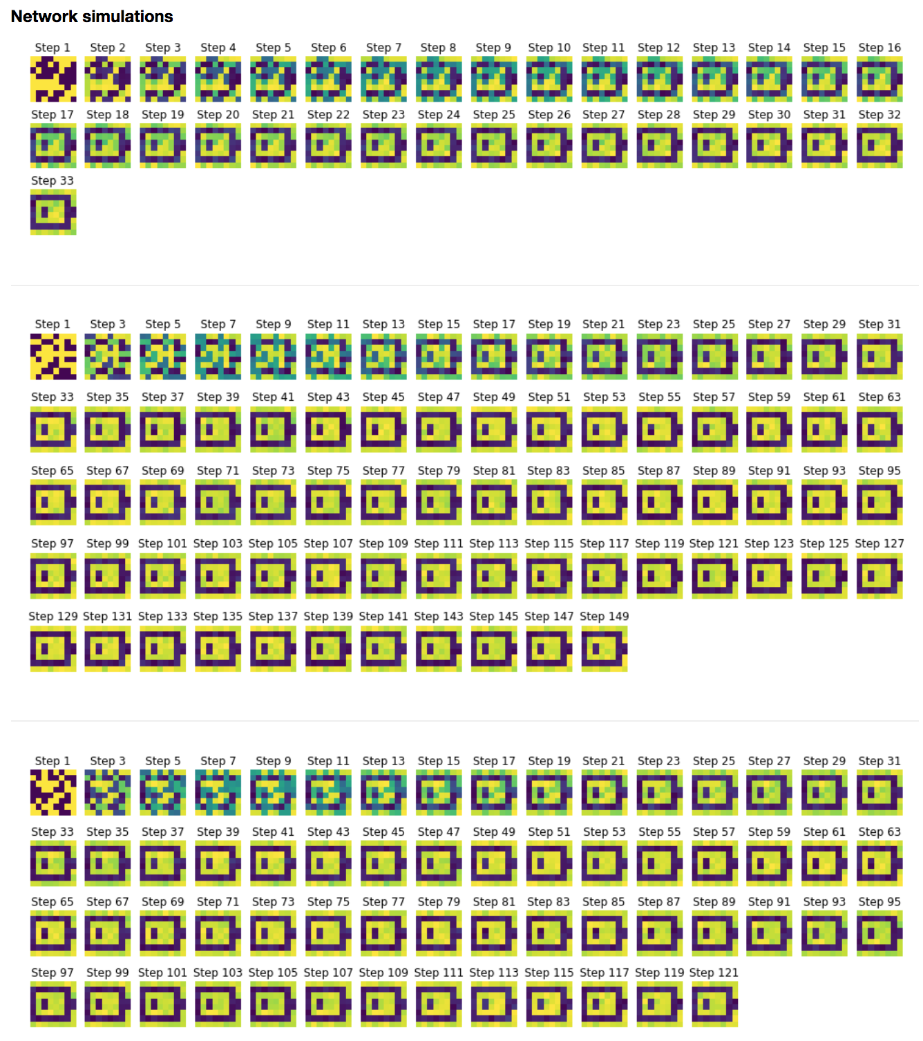
It can be noticed that the network relaxes to two fixed points, in our examples:
- the battery pattern: $\textbf{p}_{\text{bat}}$
- and its opposite pattern: $-\textbf{p}_{\text{bat}}$
From a theoretical standpoint, this can be explained by the fact that both $\textbf{p}{\text{bat}}$ and $-\textbf{p}{\text{bat}}$ are fixed points of the function
\[\textbf{x} ⟼ \sign(W\textbf{x})\]Indeed:
\[\begin{align*} \sign\left(W \textbf{p}_{\text{bat}}\right) & = \sign\left(\frac 1 N \left(\textbf{p}_{\text{bat}} {\textbf{p}_{\text{bat}}}^\T\right) \textbf{p}_{\text{bat}}\right) \\ & = \sign\left(\frac 1 N \textbf{p}_{\text{bat}} \left({\textbf{p}_{\text{bat}}}^\T \textbf{p}_{\text{bat}}\right)\right) &&\text{(because the matrix product is associative)}\\ &= \sign\Bigg(\frac 1 N \textbf{p}_{\text{bat}} \overbrace{\Bigg(\sum\limits_{ i=1 }^N \underbrace{ \left[\textbf{p}_{\text{bat}}\right]_i^2}_{= \; 1}\Bigg)}^{= \; N}\Bigg) \\ &= \sign\left(\textbf{p}_{\text{bat}}\right) \\ &= \textbf{p}_{\text{bat}} &&\text{(because } \textbf{p}_{\text{bat}} ∈ 𝔐_{N,1}(\lbrace -1, 1 \rbrace)\\ & &&\;\text{ so } \sign\left(\left[\textbf{p}_{\text{bat}}\right]_i\right) = \left[\textbf{p}_{\text{bat}}\right]_i \quad ∀1≤i≤N \text{ )} \end{align*}\]And:
\[\begin{align*} \sign\left(W (-\textbf{p}_{\text{bat}})\right) & = \sign\left(-W \textbf{p}_{\text{bat}}\right)\\ &= -\sign\left(W \textbf{p}_{\text{bat}}\right) &&\text{(because } \sign \text{ is an odd function)}\\ &= -\textbf{p}_{\text{bat}} \end{align*}\]Therefore, leaving the noise aside, by setting:
\[φ ≝ \textbf{x} ⟼ -\textbf{x} + \sign(W\textbf{x})\]so that the corresponding dynamics without noise is given by:
\[\dot{\textbf{x}} = φ(\textbf{x})\]it follows that:
\[φ(\textbf{p}_{\text{bat}}) = φ(-\textbf{p}_{\text{bat}}) = \textbf{0}\]As a result: $\textbf{p}{\text{bat}}$ and $-\textbf{p}{\text{bat}}$ are fixed points of the corresponding deterministic (i.e. without noise) dynamics, as a result of which the stochastic dynamics relaxes to them.
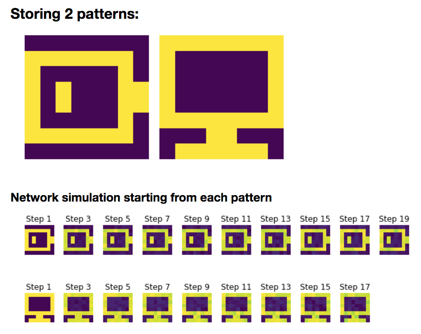
2. Storing two patterns
Now, let us add a new pattern $\textbf{p}_{\text{com}}$:
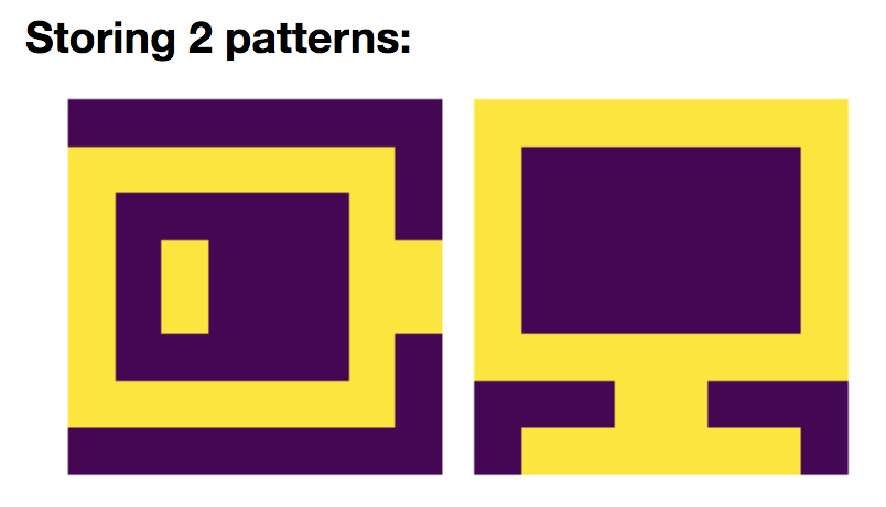
so that
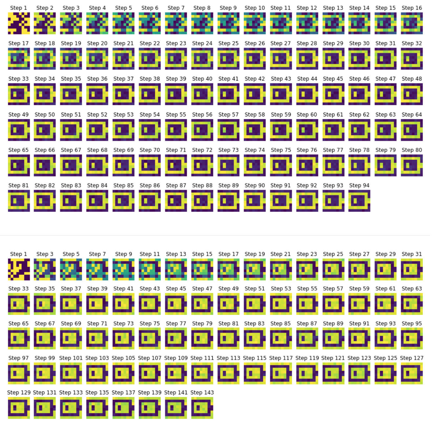
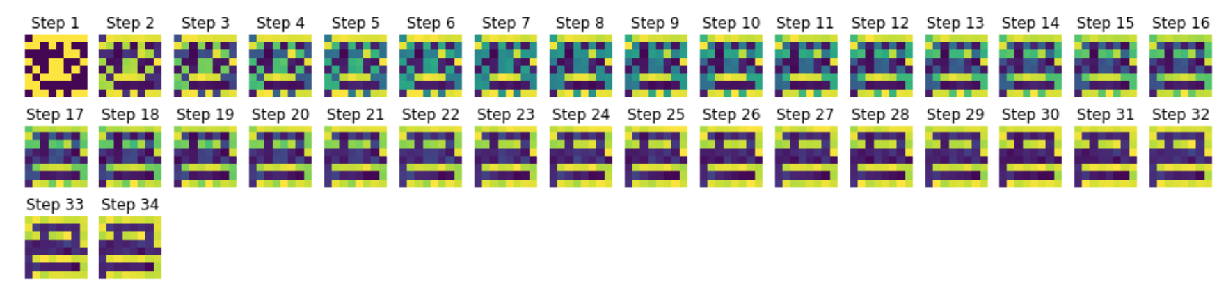
\[W = \frac 1 N \left(\textbf{p}_{\text{bat}}\textbf{p}_{\text{bat}}^\T + \textbf{p}_{\text{com}}\textbf{p}_{\text{com}}^\T\right)\]And we simulate the network on random starting patterns:
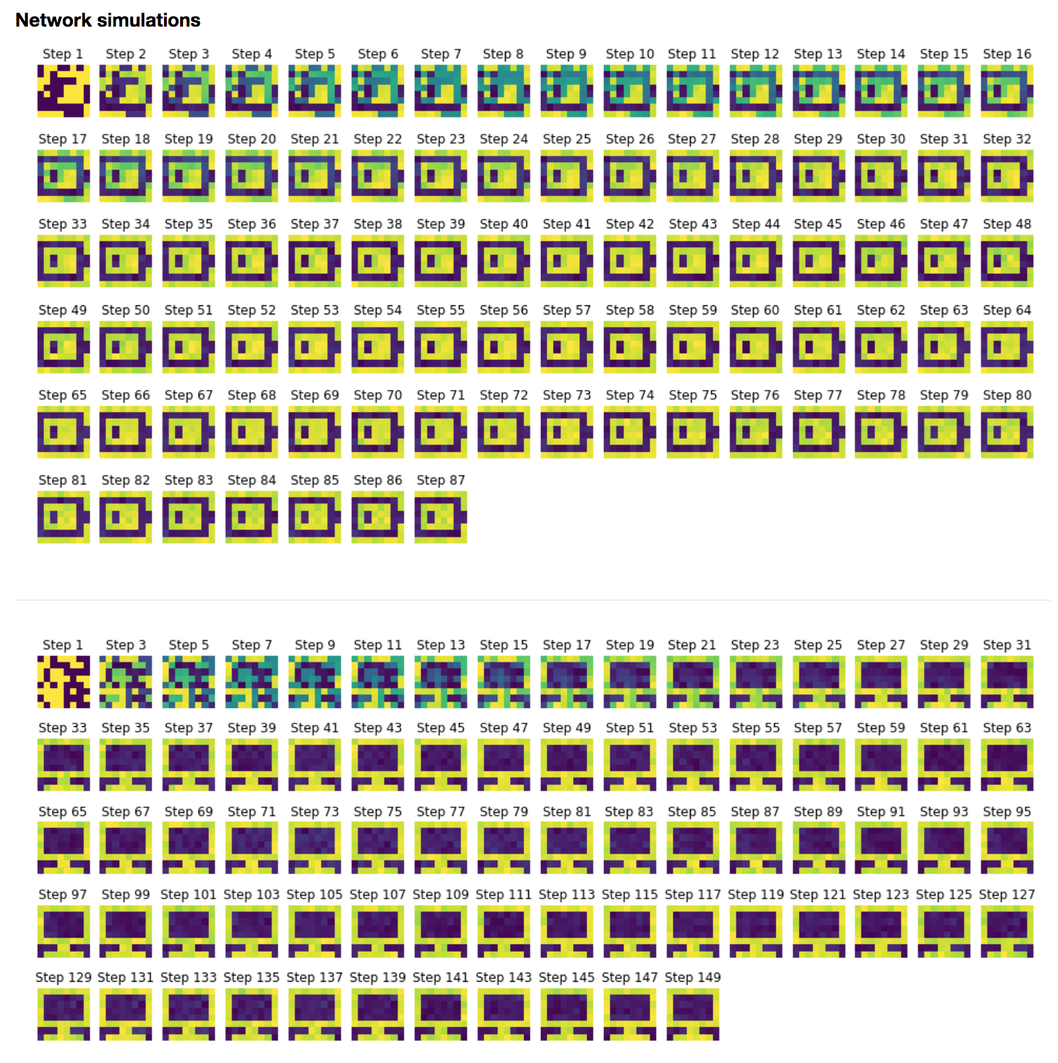
Again, we can show that:
- the battery pattern $\textbf{p}{\text{bat}}$ and its opposite pattern: $-\textbf{p}{\text{bat}}$
- the computer pattern $\textbf{p}{\text{com}}$ and its opposite pattern: $-\textbf{p}{\text{com}}$
are stored, owing to the fact that they are fixed points of the corresponding deterministic dynamics.
Indeed (for the sake of convenience, we set $\textbf{p} ≝ \textbf{p}{\text{bat}}$ and $\textbf{q} ≝ \textbf{p}{\text{com}}$):
\[\begin{align*} \sign\left(W \textbf{p}\right) & = \sign\left(\frac 1 N \left(\textbf{p} \textbf{p}^\T + \textbf{q} \textbf{q}^\T\right) \textbf{p}\right) \\ & = \sign\Big(\underbrace{\frac 1 N \left(\textbf{p} \textbf{p}^\T\right) \textbf{p}}_{\rlap{= \; \textbf{p} \; \text{(cf. previously)}}} + \frac 1 N \left(\textbf{q} \textbf{q}^\T\right) \textbf{p}\Big)\\ & = \sign\Big(\textbf{p} + \frac 1 N \, \textbf{q} \underbrace{\left(\textbf{q}^\T \textbf{p}\right)}_{\rlap{= \; ⟨\textbf{q},\, \textbf{p}⟩}}\Big)\\ \end{align*}\]But:
\[\vert ⟨\textbf{q},\, \textbf{p}⟩ \vert \, = \, \Bigg\vert \sum\limits_{ i = 1}^N \underbrace{[\textbf{q}]_i [\textbf{p}]_i}_{∈ \lbrace -1, 1 \rbrace} \Bigg\vert \, ≤ \, N\]And for $ε ∈ \lbrace -1, 1 \rbrace$:
\[\begin{align*} & ⟨\textbf{q},\, \textbf{p}⟩ = ε N \\ ⟺ \quad & \sum\limits_{ i = 1}^N [\textbf{q}]_i [\textbf{p}]_i = εN \\ ⟺ \quad & \sum\limits_{ i = 1}^N \underbrace{([\textbf{q}]_i [\textbf{p}]_i - ε)}_{≤ 0 \text{ if } ε = 1 \text{ else } ≥ 0} = 0 \\ ⟺ \quad & ∀1 ≤ i ≤ N, \quad [\textbf{q}]_i [\textbf{p}]_i - ε = 0\\ ⟺ \quad & ∀1 ≤ i ≤ N, \quad [\textbf{q}]_i [\textbf{p}]_i = ε\\ ⟺ \quad & ∀1 ≤ i ≤ N, \quad [\textbf{q}]_i = ε/[\textbf{p}]_i = ε[\textbf{p}]_i &&\text{ (because } [\textbf{p}]_i ∈ \lbrace -1, 1 \text{ )} \rbrace\\ \end{align*}\]NB: alternatively, we could have used the Cauchy-Schwarz inequality:
\[\vert ⟨\textbf{q},\, \textbf{p}⟩ \vert ≤ \underbrace{\Vert \textbf{q} \Vert_2 \, \Vert \textbf{p} \Vert_2}_{= \sqrt{N}\sqrt{N} = N} \quad \text{ and } \quad \Big(\vert ⟨\textbf{q},\, \textbf{p}⟩ \vert = N ⟺ \textbf{q} = ± \textbf{p} \Big)\]Here, as:
\[\textbf{q} ≠ \textbf{p} \quad \text{ and } \quad \textbf{q} ≠ -\textbf{p}\]it comes that:
\[\vert ⟨\textbf{q},\, \textbf{p}⟩ \vert < N\]Hence:
\[\begin{align*} \sign\left(W \textbf{p}\right) & = \sign\Big(\textbf{p} + \underbrace{\frac{\overbrace{⟨\textbf{q},\, \textbf{p}⟩}^{\rlap{∈ [-(N-1)\,, \,N-1] \; }}}{N}}_{∈ \, ]-1, 1[} \; \textbf{q}\Big)\\ &\overset{⊛}{=} \sign\left(\textbf{p}\right) &&\text{(because each } \frac {⟨\textbf{q},\, \textbf{p}⟩} N \, [\textbf{q}]_i ∈ \left[-1 + \frac 1 N, \, 1-\frac 1 N \right]\\ & && \quad \text{: it can't change the sign of } [\textbf{p}]_i ∈ \lbrace -1, 1 \rbrace\text{ )} \\ &= \textbf{p} \end{align*}\]And likewise, by symmetry:
\[\sign\left(W \textbf{q}\right) = \textbf{q}\]Once we know that $\textbf{p}$ and $\textbf{q}$ are fixed points, the same holds true for their opposites, as $\sign$ is an odd function (the proof is the same as previously).
So $±\textbf{p}$ and $±\textbf{q}$ are all fixed points of the corresponding deterministic dynamics, as a result of which the stochastic dynamics relaxes to them.
NB: in the computations, the key point is the equality $⊛$, which stems from $\textbf{q}$ being different from $±\textbf{p}$ (by Cauchy-Schwarz).
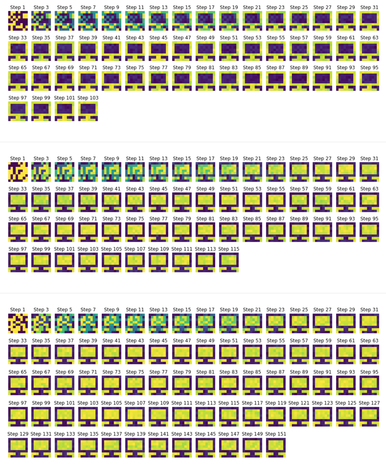
On top of that, it can be noted that the network relaxes to the fixed-point pattern which is the closest to the starting pattern! For example, consider the second-to-last and the third-to-last examples in figure 2.c.2:
- for both of these examples, in the starting pattern, we can distinguish what looks like the base of a (future) screen
- but the the second-to-last example converges to a bright-screen computer, whereas the third-to-last converges to a dark-screen one. This can be accounted for by the fact that there are more dark pixels in the third-to-last starting pattern than in the second-to-last one!
Therefore, we begin to see why Hopfield networks can be thought of as modeling an associative memory-like process: the starting patterns are similar to “visual clues”, to which the network associates the best (i.e. the closest) matching stored pattern.
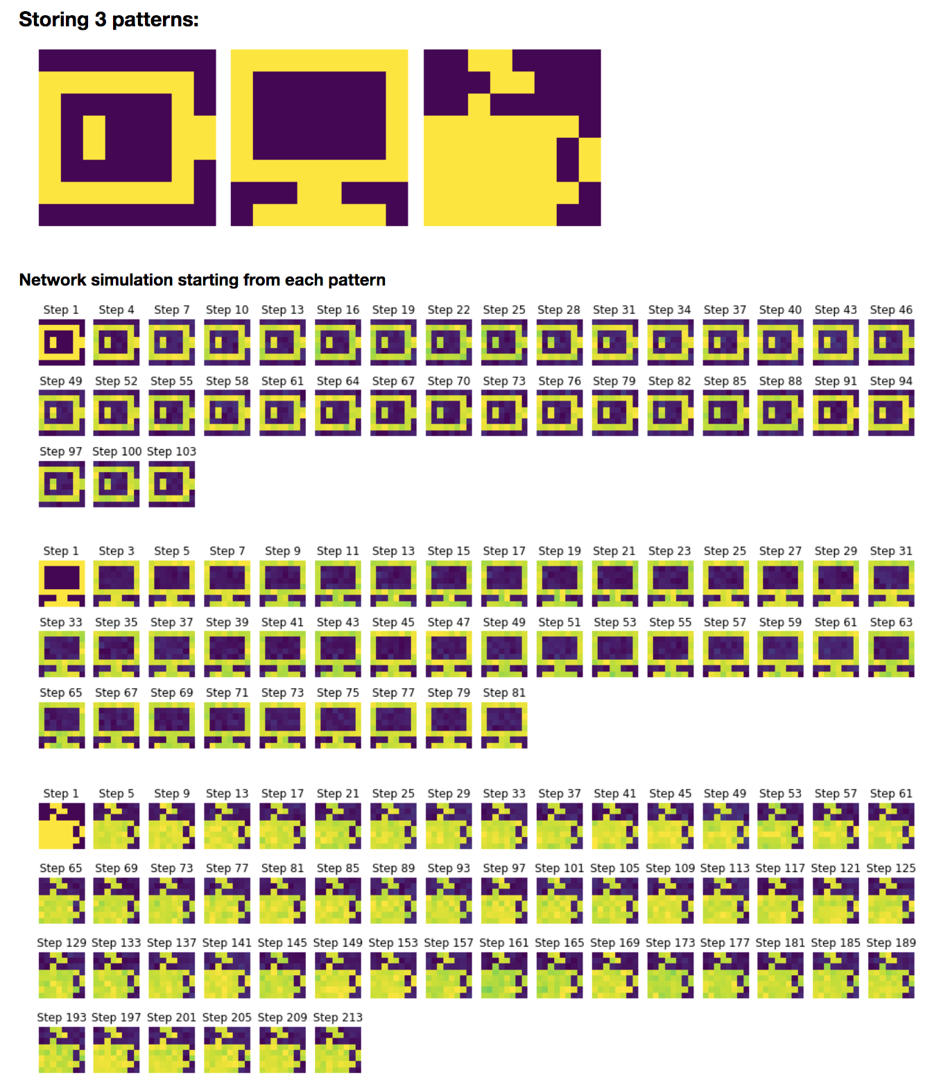
3. The general rule
The general rule defining the weight matrix is:
\[W ≝ \frac 1 N \sum_{i=1}^M \textbf{p}_i \textbf{p}_i^\T\]where the $\textbf{p}_i$ are the patterns to be stored.
3 patterns: linear combinations stored
Let us add yet another pattern: $\textbf{p}_{\text{cof}}$:
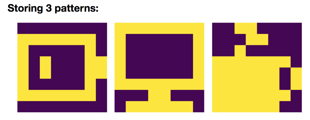
so that, in compliance with the general rule:
\(W = \frac 1 N \left(\textbf{p}_{\text{bat}}\textbf{p}_{\text{bat}}^\T + \textbf{p}_{\text{com}}\textbf{p}_{\text{com}}^\T + \textbf{p}_{\text{cof}}\textbf{p}_{\text{cof}}^\T\right)\)
Then, we simulate the network with random initial conditions: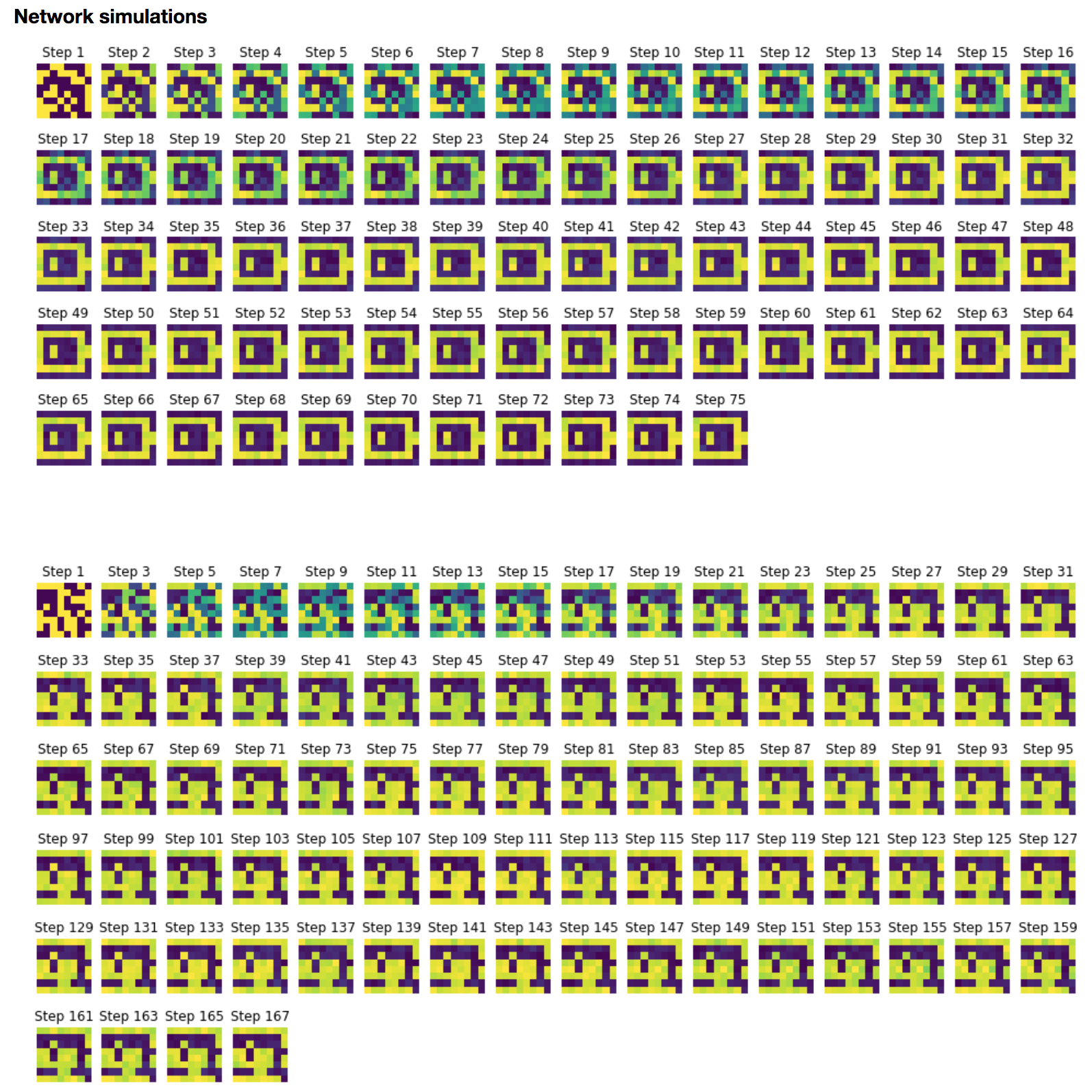
It appears that the networks relaxes to the following linear combinations of $\lbrace \textbf{p}_{\text{bat}}, \textbf{p}_{\text{com}}, \textbf{p}_{\text{cof}} \rbrace$ too:
- \[\textbf{p}_{\text{bat}} - \textbf{p}_{\text{com}} - \textbf{p}_{\text{cof}}\]
- \[\textbf{p}_{\text{bat}} - \textbf{p}_{\text{com}} + \textbf{p}_{\text{cof}}\]

So: on top of the patterns from which the weight matrix is constructed and their opposites, linear combinations thereof may also be stored.
Storing capacity
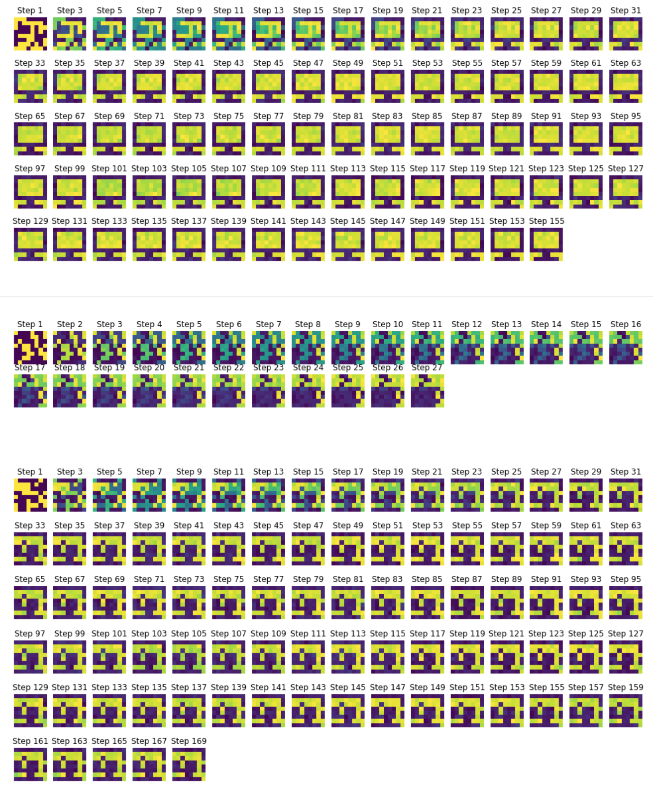
Finally, we will investigate how many patterns we can store in this $N=64$ neurons network by:
- adding new patterns, one after another
- and then simulating the network with each pattern as initial condition to see if the pattern is stored or not
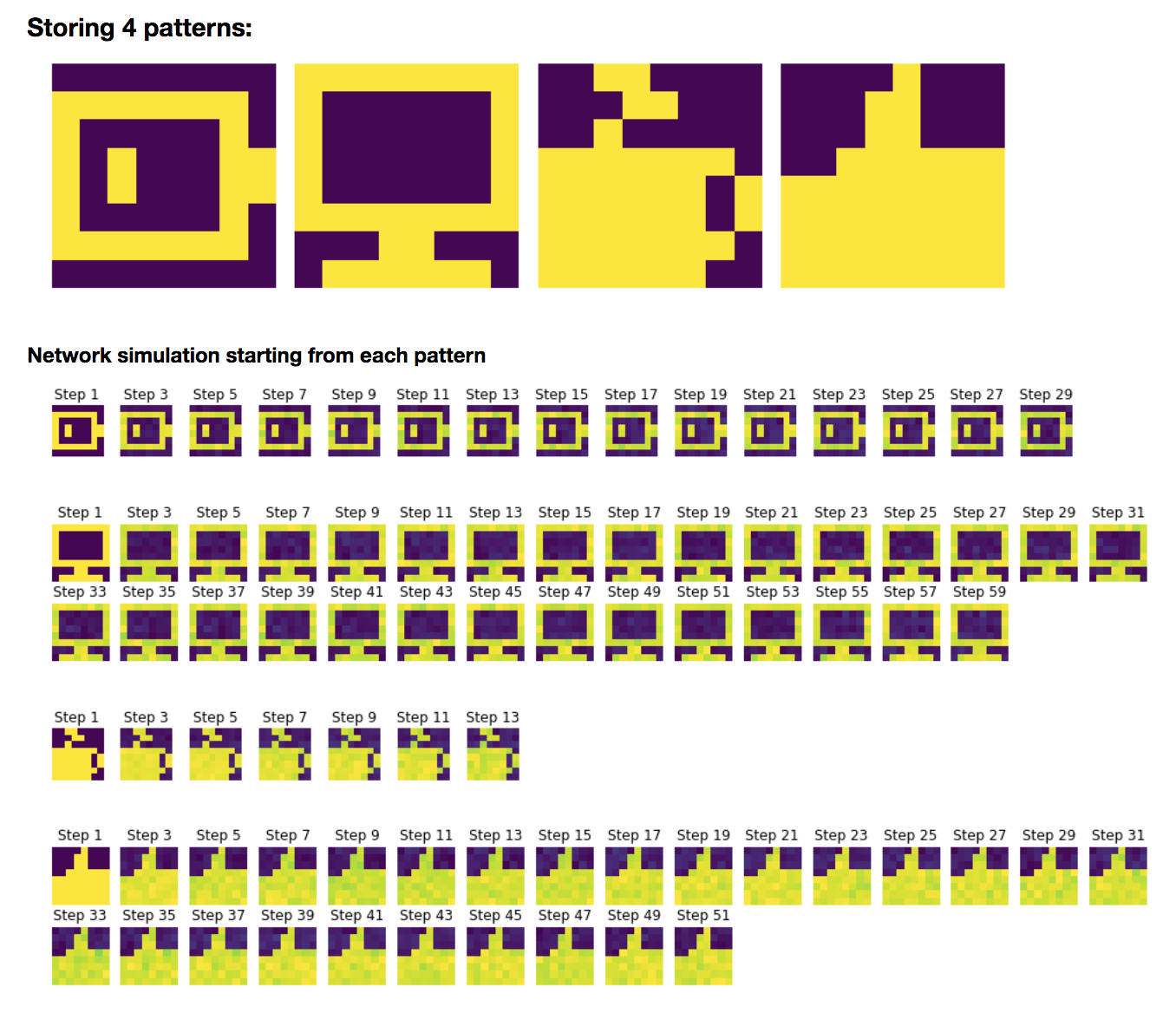
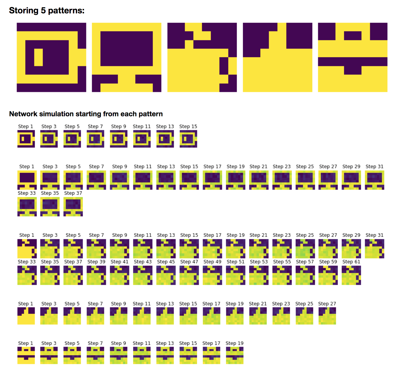
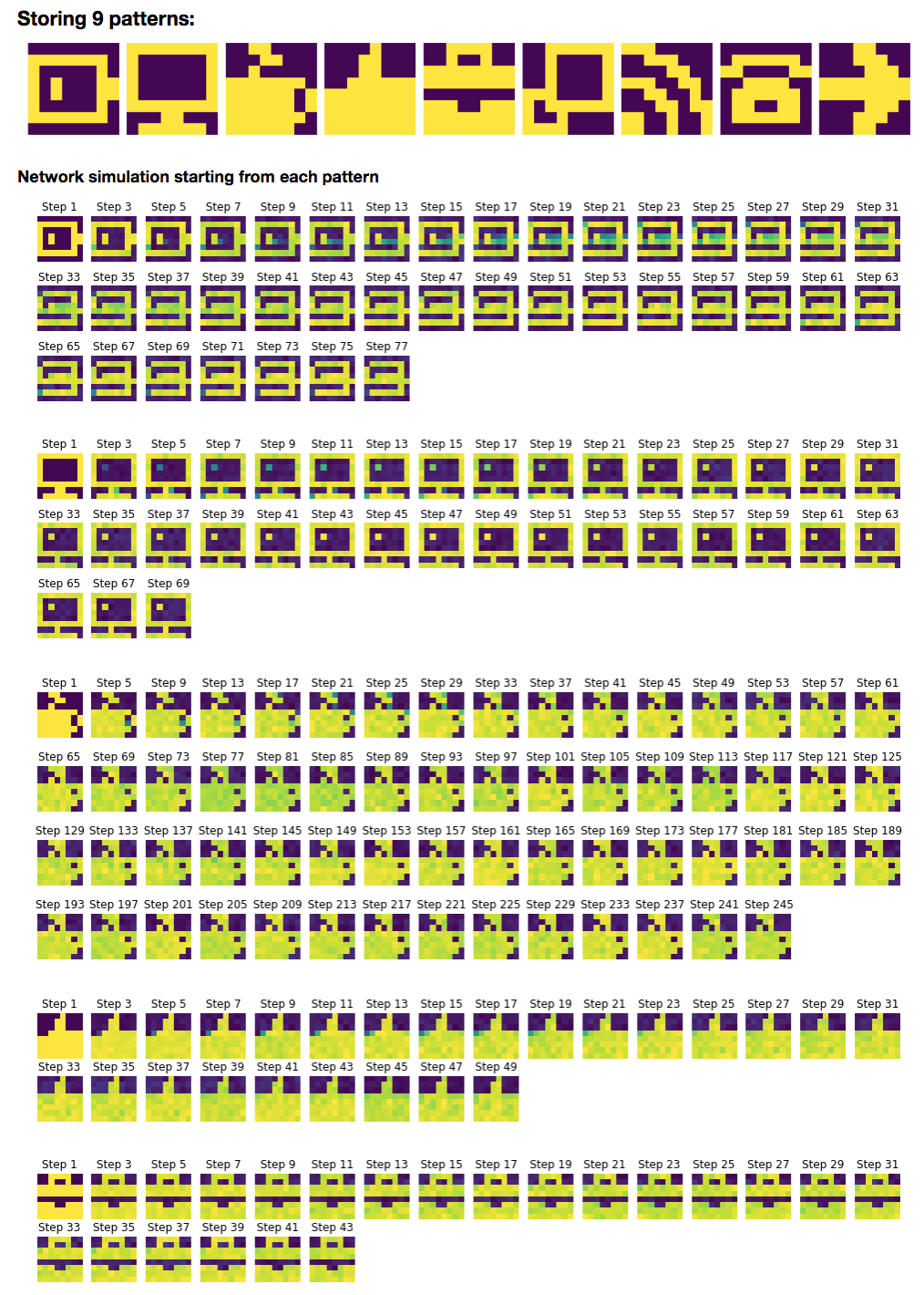
As a consequence:
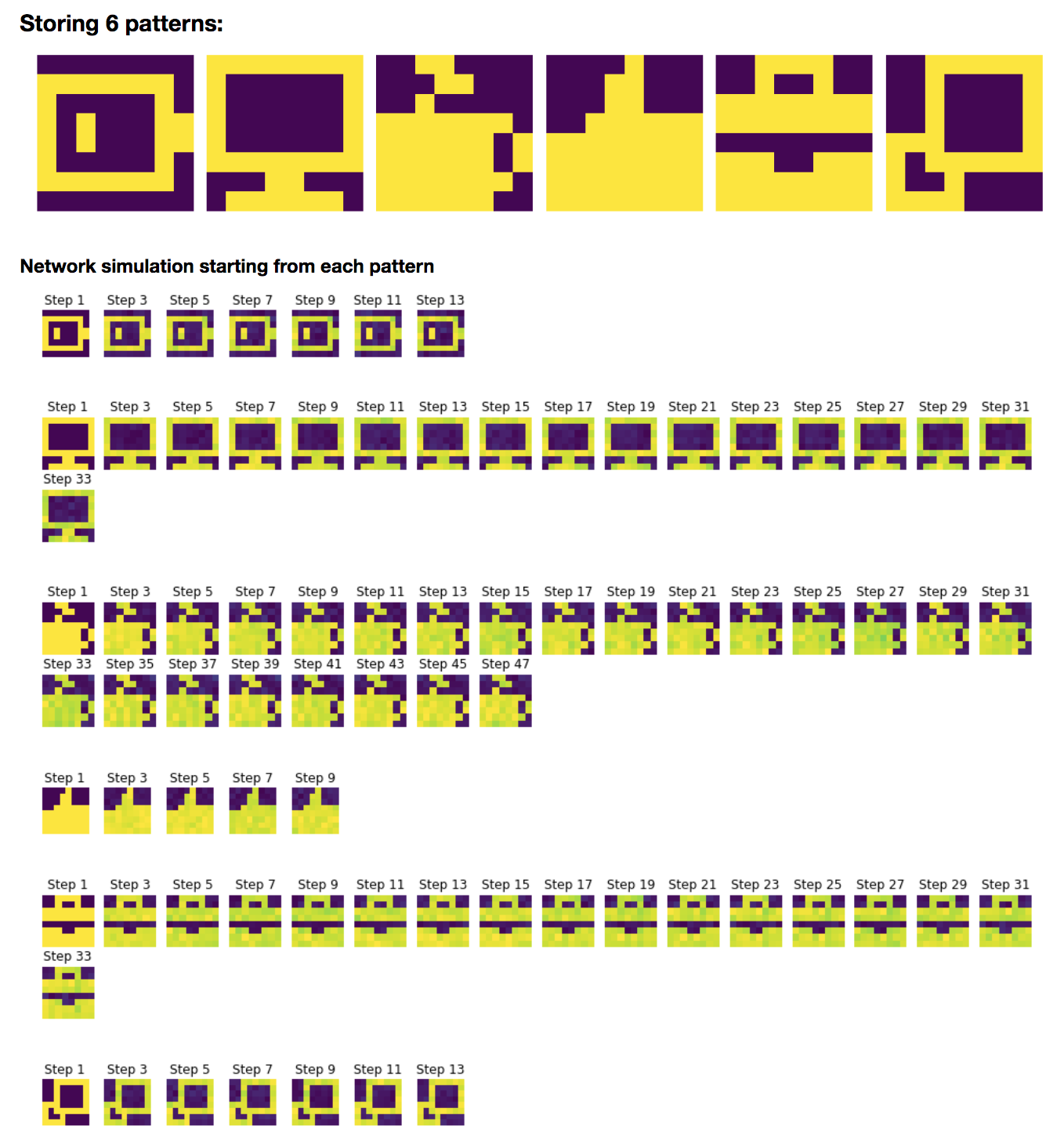
- up until 6 (included) patterns: all the patterns are successfully stored
-
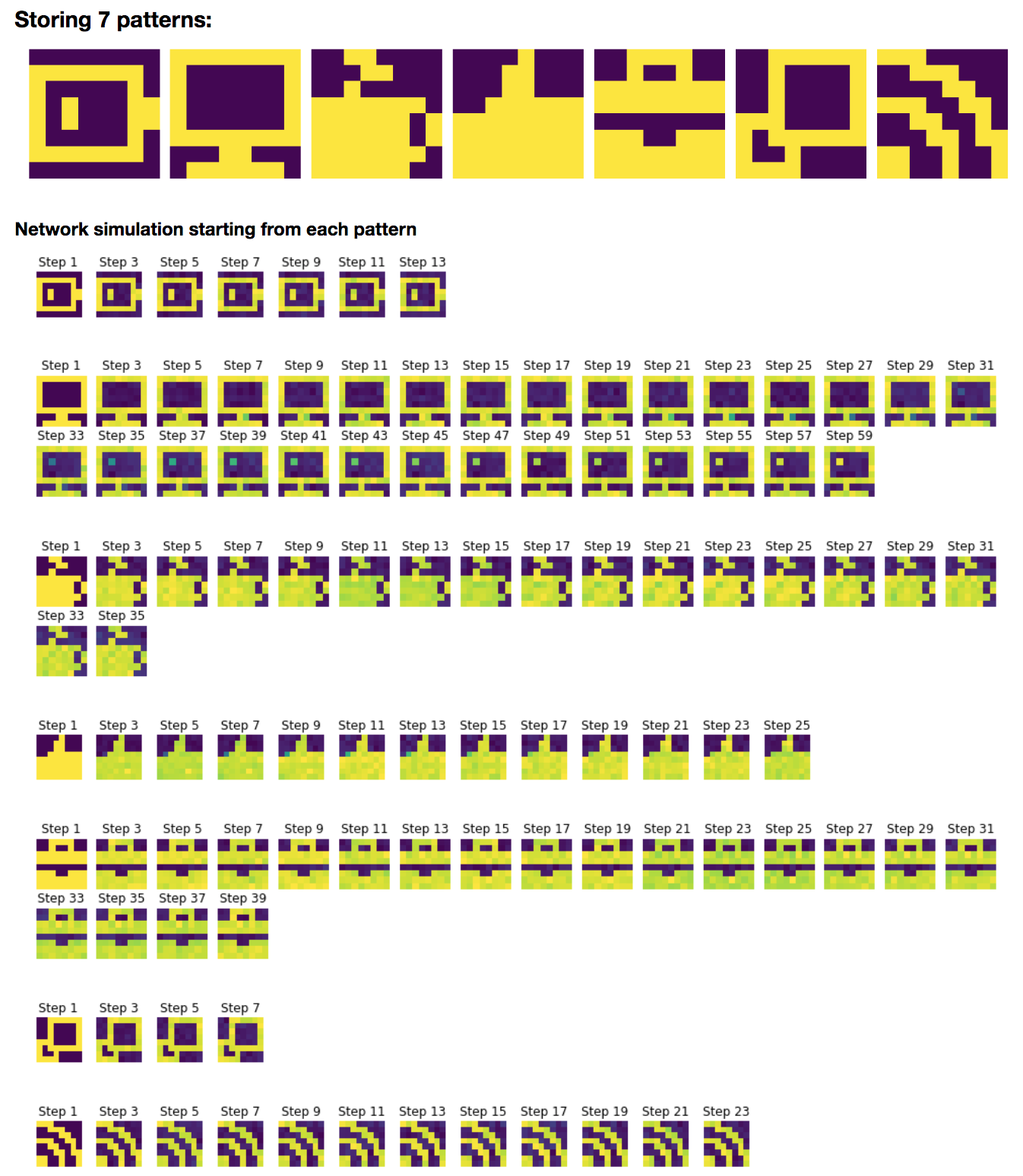
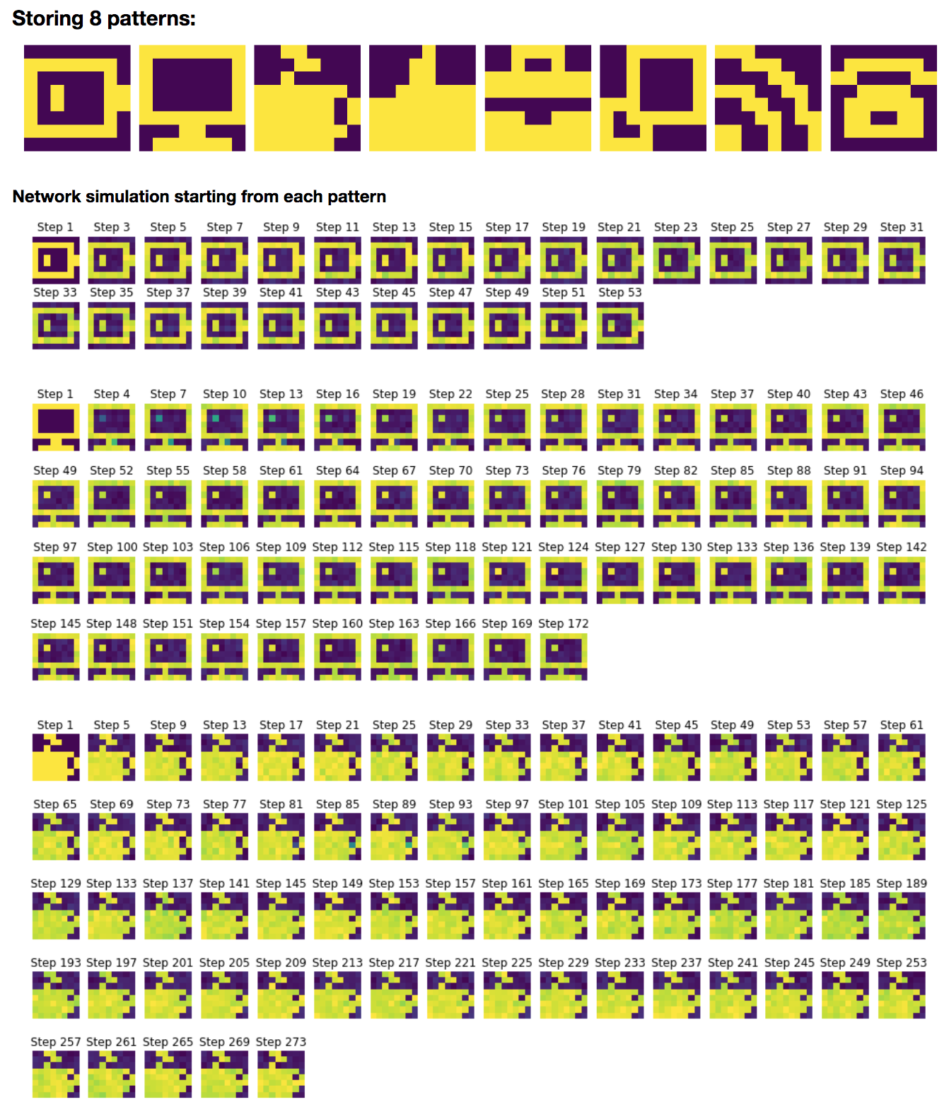
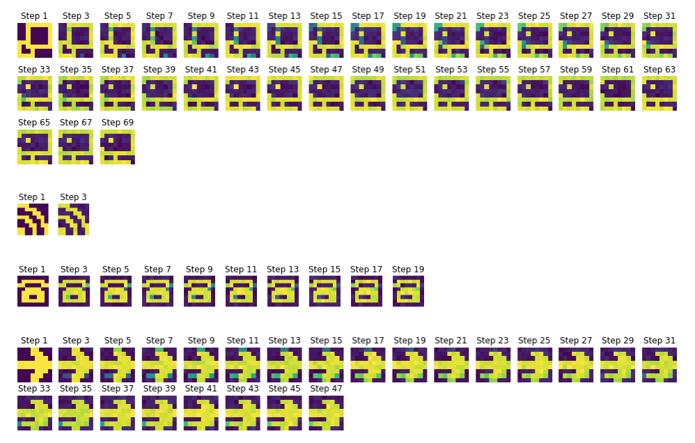
from 7 pattern on, some are not properly stored, and it gets worse and worse as the number of patterns increases:
- with 7 patterns: the computer screen is “prettified by bright pixels” (looking like light reflection!), but not stored unaltered
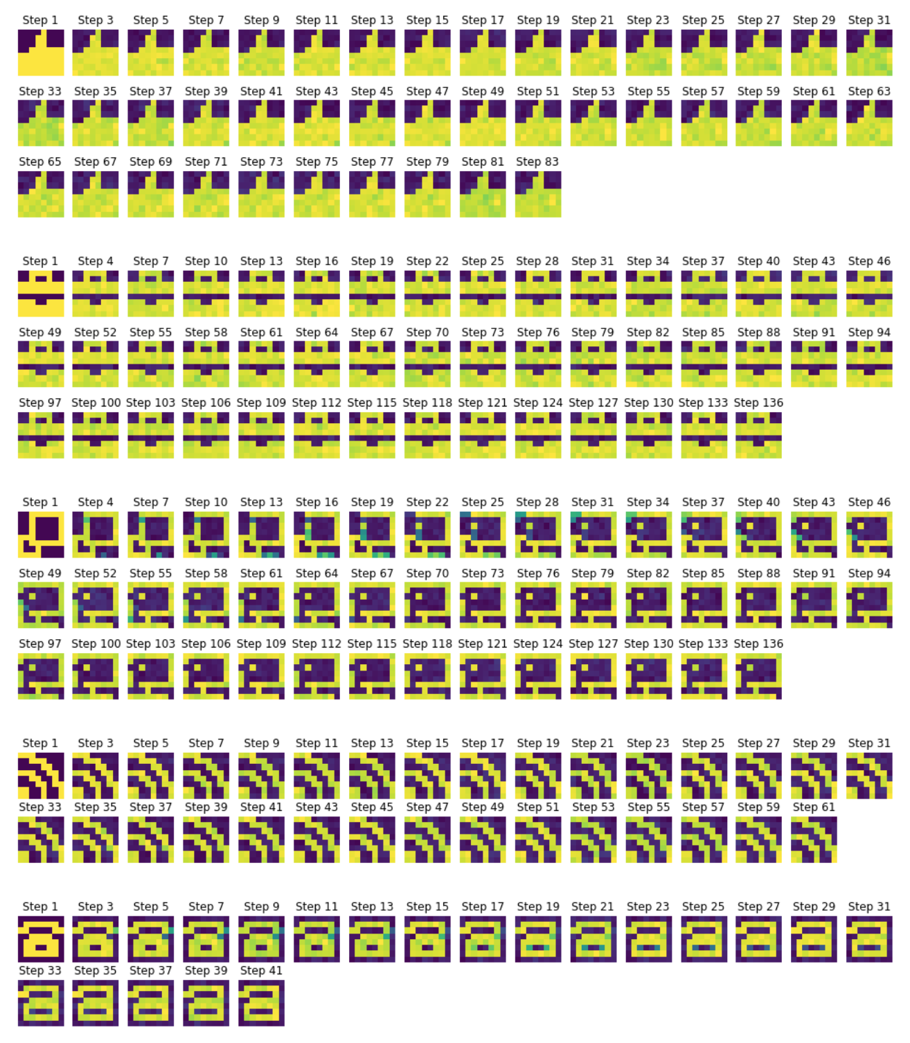
- with 8 patterns: on top of the light reflection on the computer screen, the copy icon is not stored at all: the network converges to an out-of-shape computer screen. In the same vein, the phone pattern ends up being deformed.
- with 9 patterns: the battery pattern is not stored anymore, the computer base is shifted, the cup of coffee, the thumbs up, the phone and the arrow are distorted, and the copy icon keeps converging toward the computer (they must look too similar for the full network’s pattern memory).
On the whole: the $64$-neurons Hopfield network can perfectly store $6$ patterns (and almost $7$ patterns, if it were not for the computer pattern ending up with a few bright pixels on the screen).
Leave a comment