Problem Set 4: Networks
AT2 – Neuromodeling: Problem set #4 NETWORKS
Younesse Kaddar
PROBLEM 1: Neuron with Autapse
Link of the iPython notebook for the code
1. One-dimensional deterministic dynamical system
Let us consider a neuron whose axons connects to its own dendrites (the resulting synapse is called an autapse): we will denote by
- $x$ its firing rate
- $w = 0.04$ the strength of the synaptic connection
- $I = -2$ an external inhibitory input
-
$f(s) ≝ 50 \, (1 + \tanh(s))$ the neuron’s activation function, where $s$ is the overall neuron input:
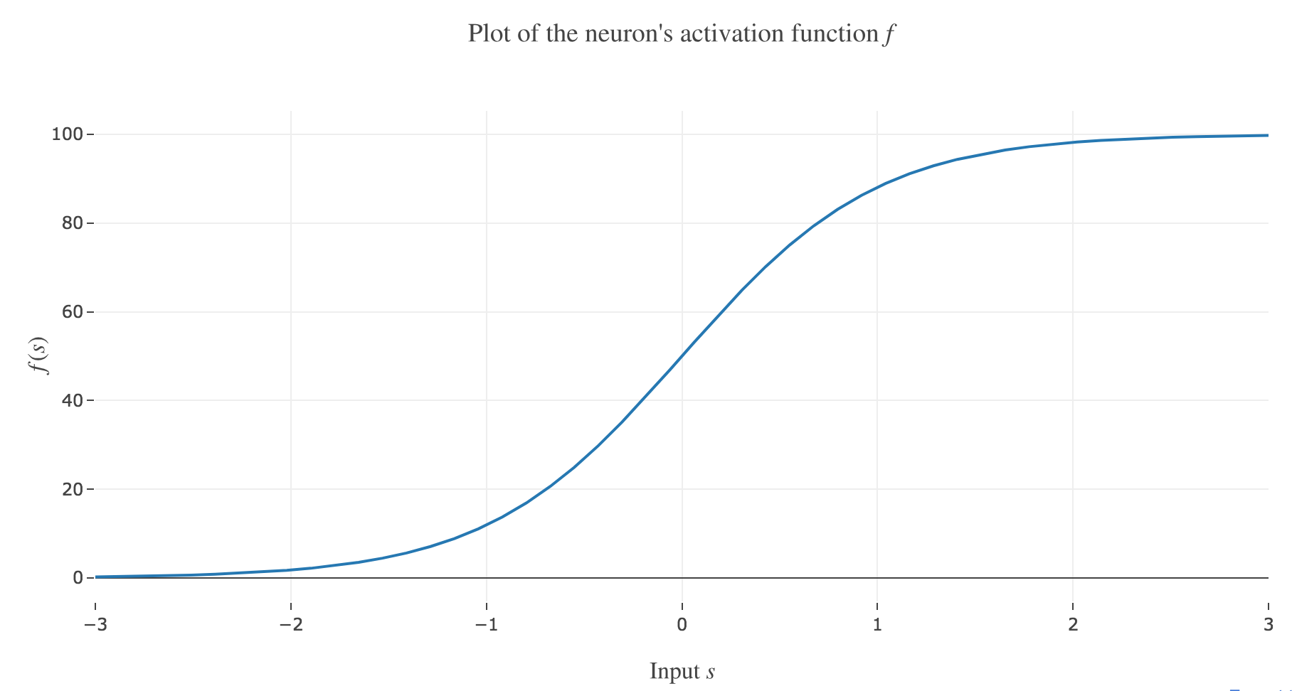
Figure 1.a. - Plot of the neuron's activation function $f$
(in arbitrary units) so that the firing rate is described by the following differential equation:
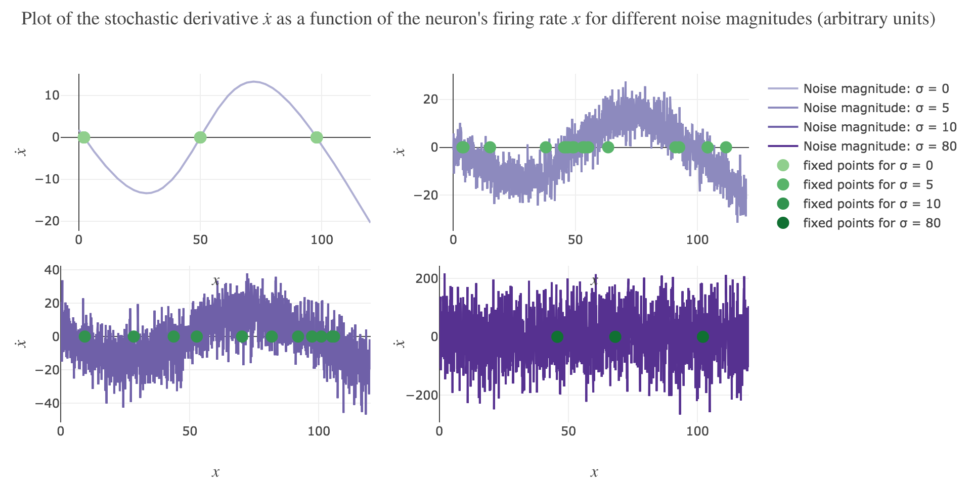
\[\dot{x}(t) = - x(t) + f\big(wx(t) + I\big)\]Plotting the derivative $\dot{x}$ as a function of the neuron’s firing rate $x$:
\[x ⟼ - x + f\big(wx + I\big)\]results in the following 1-dimensional system dynamics:
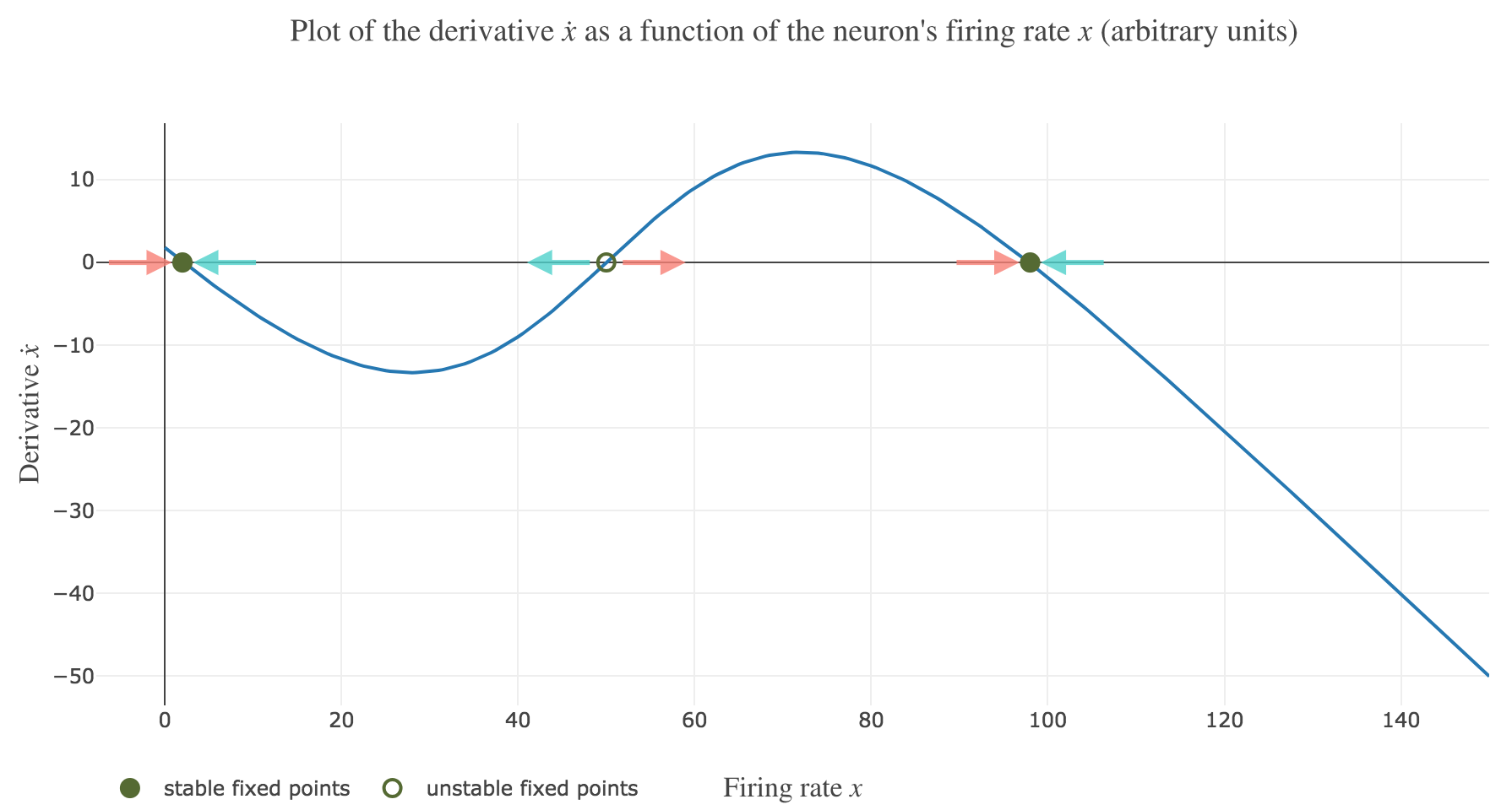
The zero-crossings of $\dot{x}$ as a function of $x$ correspond to critical points, i.e. values of $x$ at which the derivative $t ⟼ \dot{x}(t)$ equals zero, hence the function $t ⟼ x(t)$ being constant with respect to $t$. As a consequence, such values of $x$ at which $\dot{x}$ (as a function of $x$) vanishes are called fixed point of the dynamics, as $x$ is left unchanged over time.
Dynamics fixed points are twofold:
-
stable fixed points (attractors) are fixed points around which a slight change of $x$ leads to $x$ moving back to the stable fixed point value: these correspond to points $x^\ast$ such that the derivative $\dot{x}$ is:
- positive at $x^\ast-ε$ ($x$ increases back to $x^\ast$)
- negative at $x^\ast+ε$ ($x$ decreases back to $x^\ast$)
for $ε>0$ sufficiently small. In other words, the zero-crossing goes from positive values to negative ones.
On Figure 1.b., the two stable fixed points at $x=2$ and $x=98$ are indicated by a filled up green point.
-
unstable fixed points (repellers) are fixed points around which a slight change of $x$ leads to $x$ moving away from the unstable fixed point value: these correspond to points $x^\ast$ such that the derivative $\dot{x}$ is:
- negative at $x^\ast-ε$ ($x$ keeps decreasing away from $x^\ast$)
- positive at $x^\ast+ε$ ($x$ keeps increasing away from $x^\ast$)
for $ε>0$ sufficiently small. In other words, the zero-crossing goes from negative values to positive ones.
On Figure 1.b., the only unstable fixed point at $x=50$ is indicated by a hollow green circle.
Now, let us simulate the system for various initial conditions:
\[x(0) ∈ \Big\lbrace \overbrace{49}^{\llap{\text{just below the unstable fixed point}}}\,, \underbrace{50}_{\text{the unstable fixed point}}, \overbrace{51}^{\rlap{\text{just above the unstable fixed point}}} \Big\rbrace\]We set (arbitrary units):
- the time-increment to integrate the differential equation with the Euler method: $dt = Δt ≝ 0.1$
- The total duration $T = 10 = 100 Δt$
so that the Euler method yields:
\[\begin{align*} \quad & \frac{x(t+Δt) - x(t)}{Δt} = - x(t) + f\big(wx(t) + I\big) \\ ⟺ \quad & x(t+Δt) - x(t) = - x(t) Δt + f\big(wx(t) + I\big) Δt \\ ⟺ \quad & x(t+Δt) = (1 - Δt) x(t) + f\big(wx(t) + I\big) Δt \end{align*}\]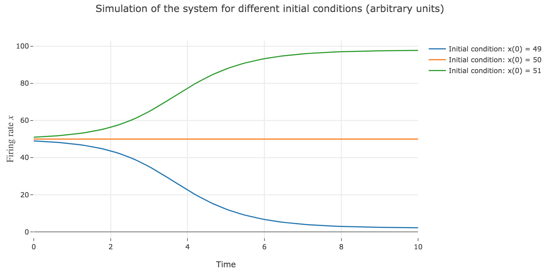
As expected, since $x=50$ is an unstable fixed point of the dynamics: when
-
$x(0) = 50$: $x(t)$ remains constantly equal to $50$ over time (as $50$ is a fixed point)
-
$x(0) = 51 > 50$: $x(t)$ keeps increasing, converging to the (stable) fixed point $98$, since the time derivative $\dot{x}$ is strictly positive at $98 > x >50$ (cf. Figure 1.b.)
-
$x(0) = 49 < 50$: $x(t)$ keeps decreasing, converging to the (stable) fixed point $2$, since the time derivative $\dot{x}$ is strictly negative at $2 < x<50$ (cf. Figure 1.b.)
2. One-dimensional stochastic dynamical system
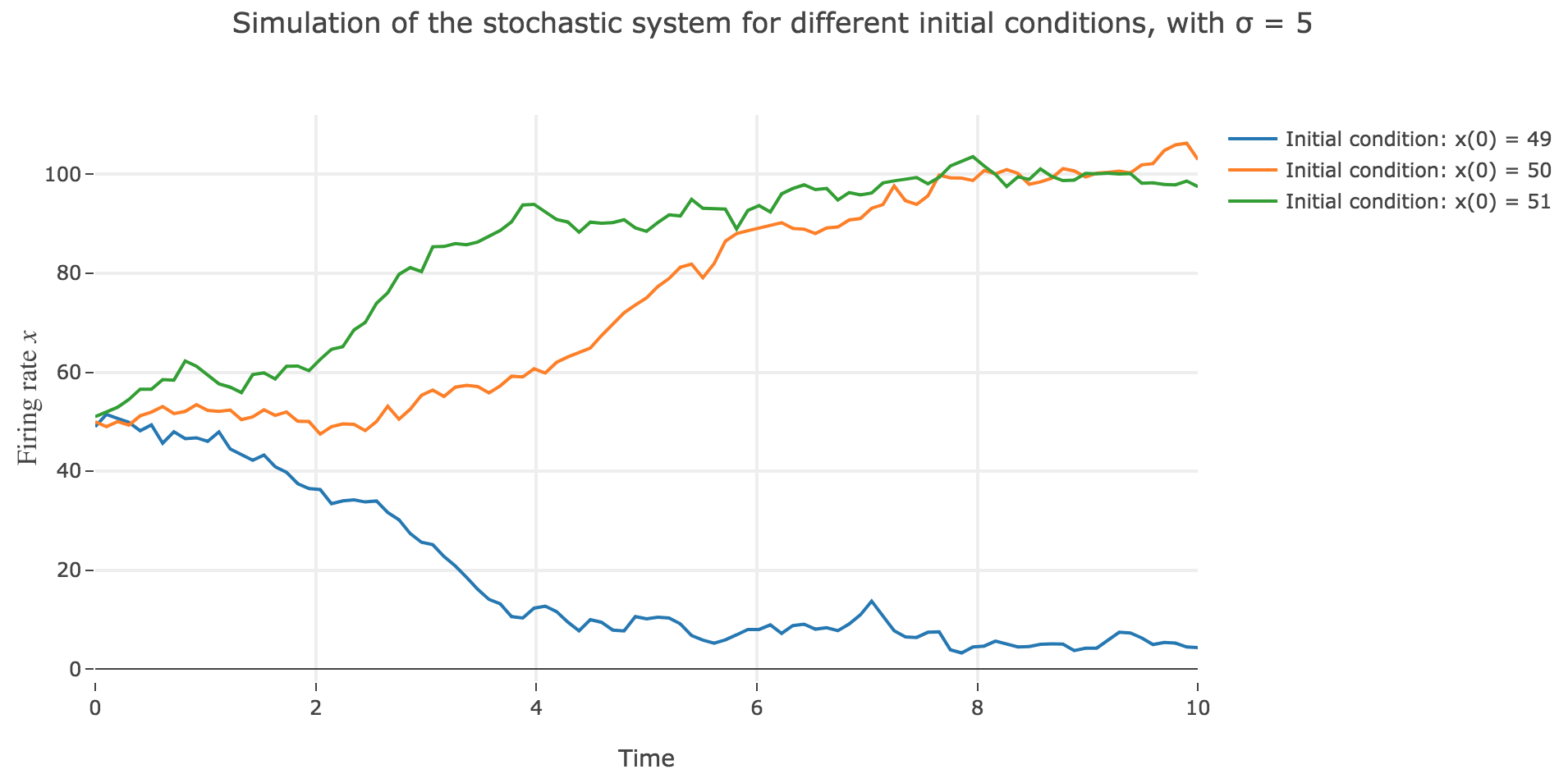
From now on, for the sake of realism, we add a white noise component to the system:
\[\dot{x}(t) = - x(t) + f\big(wx(t) + I\big) + σ η(t)\]where $η(t)$ is a Gaussian noise, $σ$ is the noise magnitude.
The stochastic differential equation is solved numerically as follows:
\[\begin{align*} \quad & x(t+Δt) - x(t) = - x(t) Δt + f\big(wx(t) + I\big) Δt + σ η(t) \sqrt{Δt} \\ ⟺ \quad & x(t+Δt) = (1 - Δt) x(t) + f\big(wx(t) + I\big) Δt + σ η(t) \sqrt{Δt} \end{align*}\]which leads to (for $σ = 5$ and several random seeds):
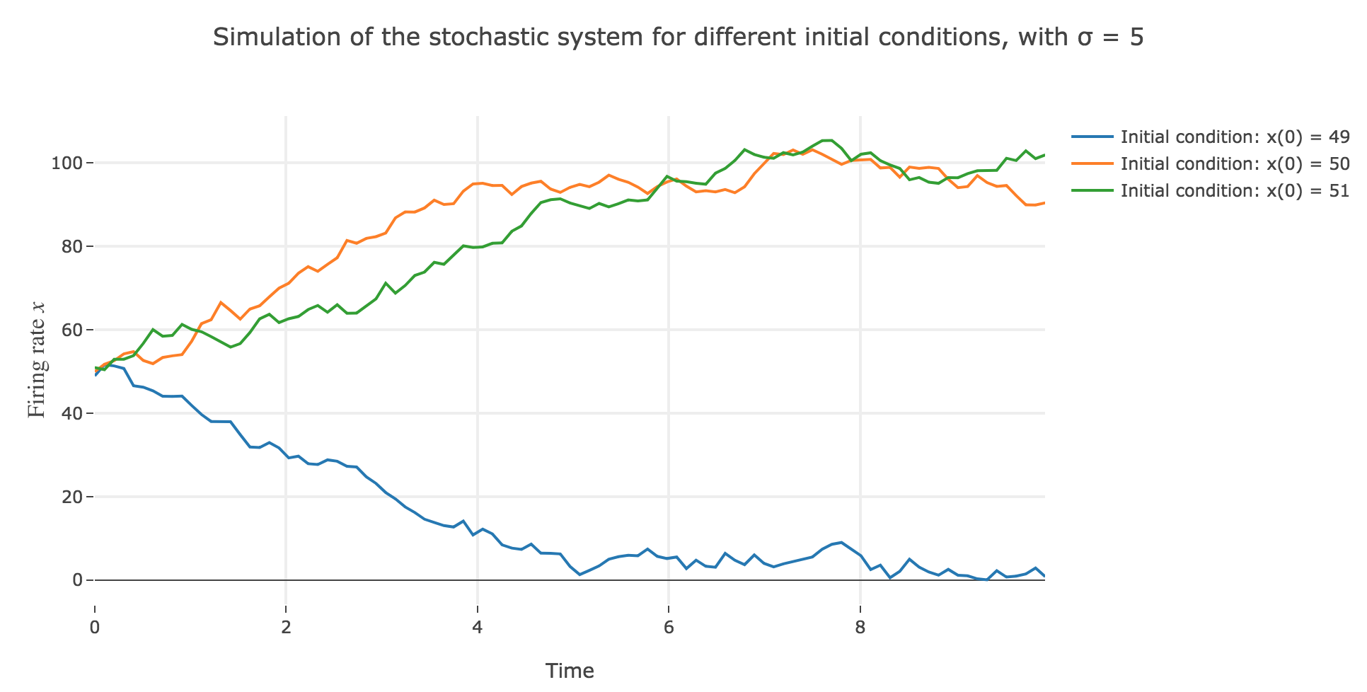
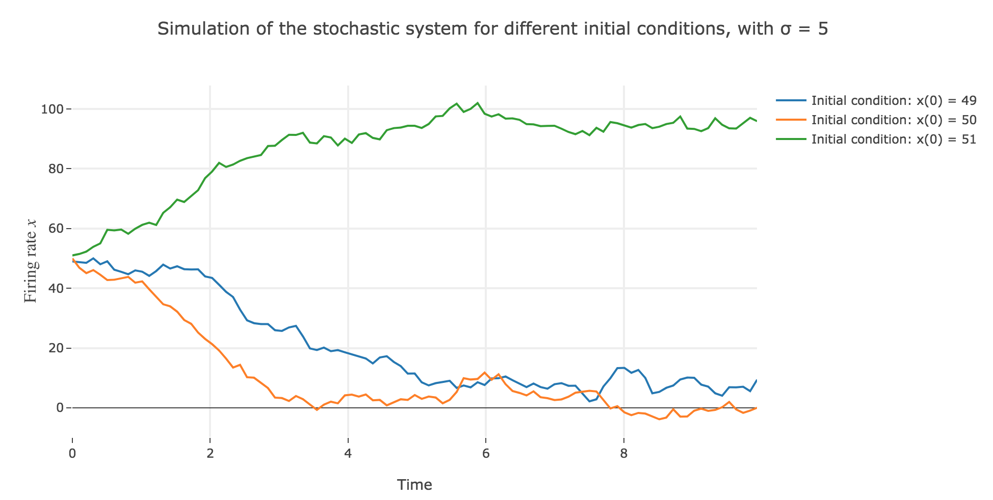
-
the $x(0)=50$ initial condition starts from an unstable fixed point of the dynamics (as seen before) when there is no noise: any slight variation of $x$ relative to this unstable fixed point leads to $x(t)$ moving away from this value. As it happens, here, this variation stems from the noise added to the time derivative $\dot{x}$, which results in the unstable fixed point being slighly moved aside, leading to $x(t)$ ending up above or below this unstable fixed point, and thus converging toward one the two stable fixed points ($2$ and $98$), depending on whether the noise variation has drawn the unstable fixed point:
- above $x$ (leading $x$ to decrease toward $2$), as in figure 2.d.1.3
- or below $x$ (leading $x$ to increase toward $98$), as in figures 2.d.1.1 and 2.d.1.2
-
the $x(0) = 49$ (resp. $x(0) = 51$) initial conditions causes $x(t)$ to decrease (resp. increase) toward the stable fixed point $2$ (resp. $98$) when there is no noise (as seen before): any slight variation of $x$ relative to these stable fixed points bring $x(t)$ back to them. The only possibility for $x$ not to converge toward $2$ (resp. $98$) instead would be that the noise added to derivative has such a magnitude that it makes it positive (resp. negative) at $x$, which doesn’t happen in the three figures 2.d.1.1, 2.d.1.2, and *2.d.1.3**: the added noise magnitude is too small: $x$ still converges toward the expected fixed point.
Now for various noise magnitudes:
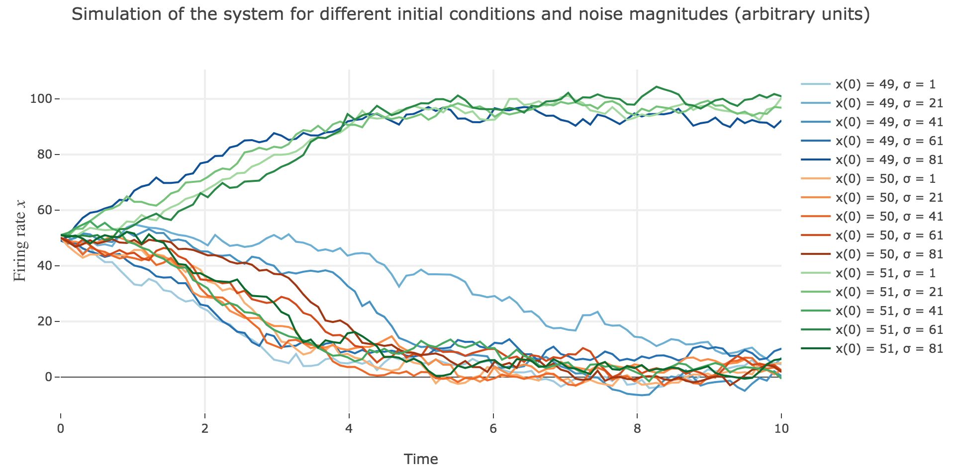
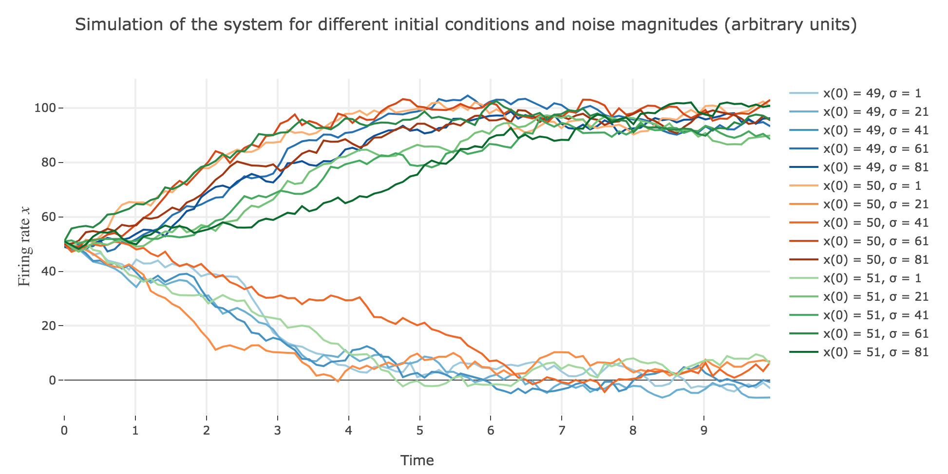
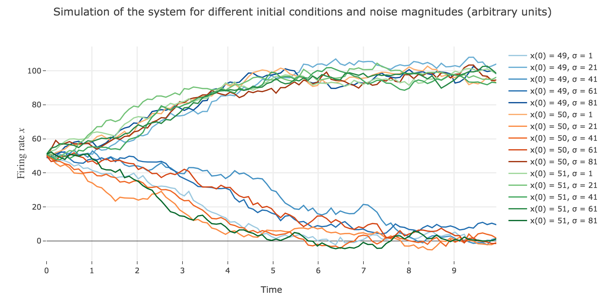
As the initial condition $x(0)=50$ starts from an unstable fixed point of the deterministic dynamics, $x$ may equiprobably converge to one the two stable fixed points when adding the noise, which makes this case of little interest (it clutters the graphs uselessly). We may as well only plot the remaining relevant cases ($x(0) ∈ \lbrace 49, 51 \rbrace$):
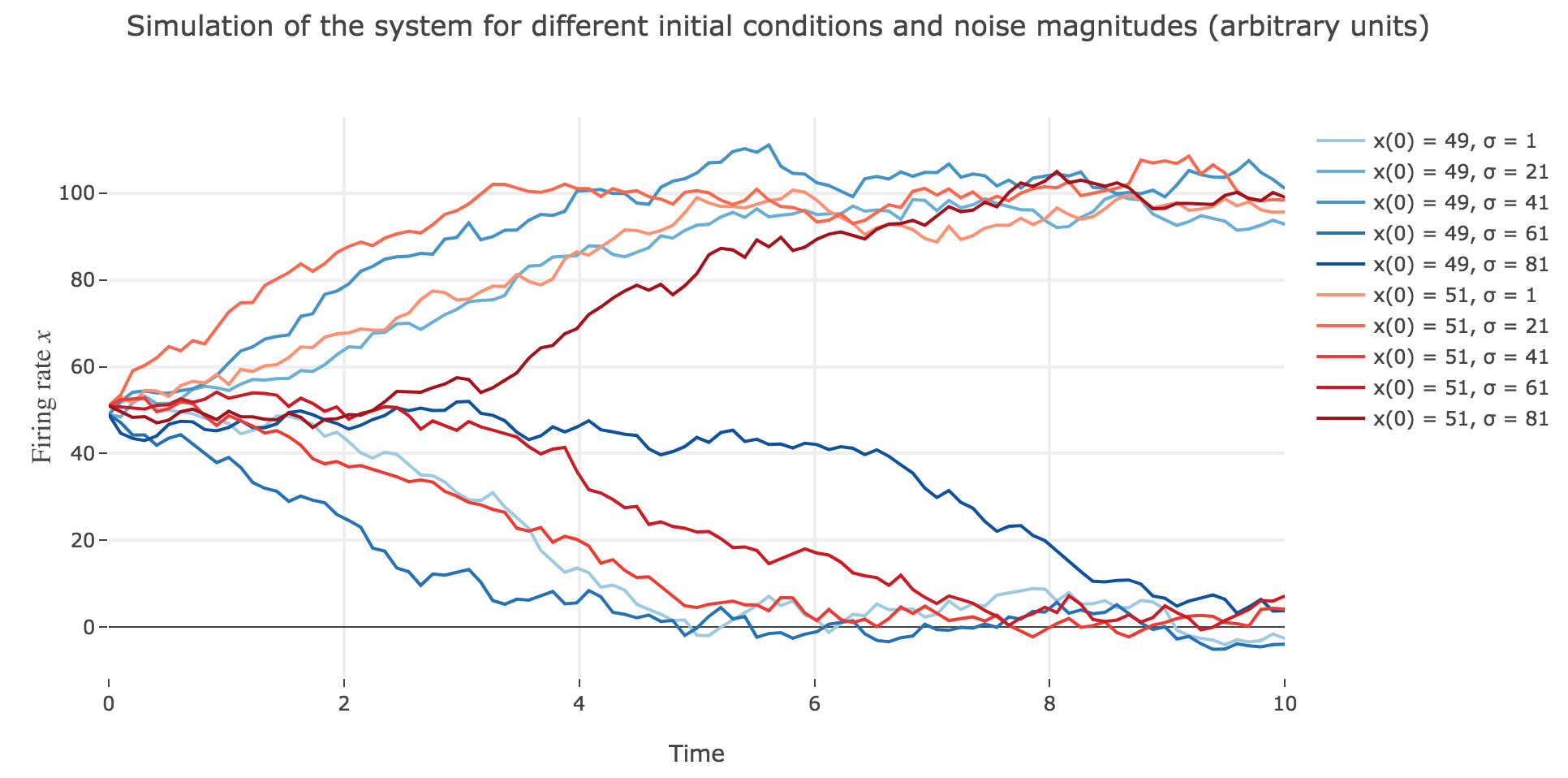
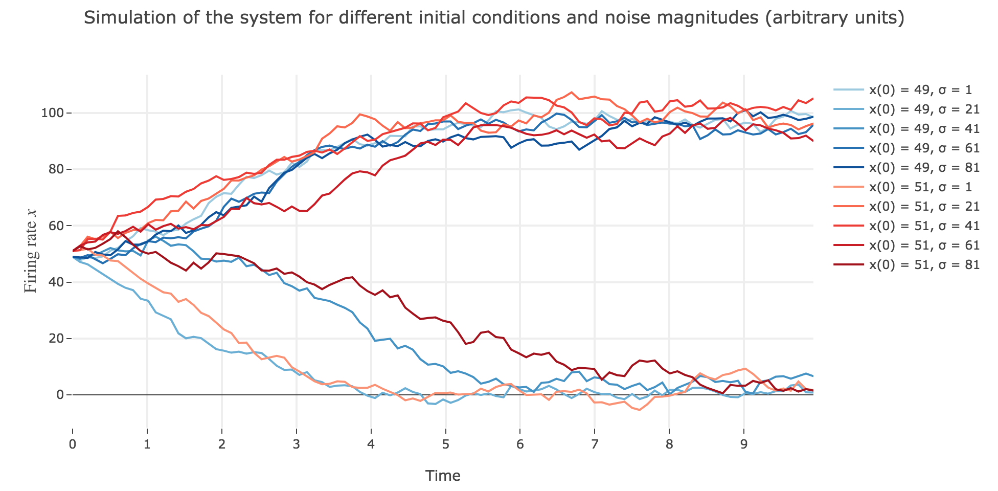
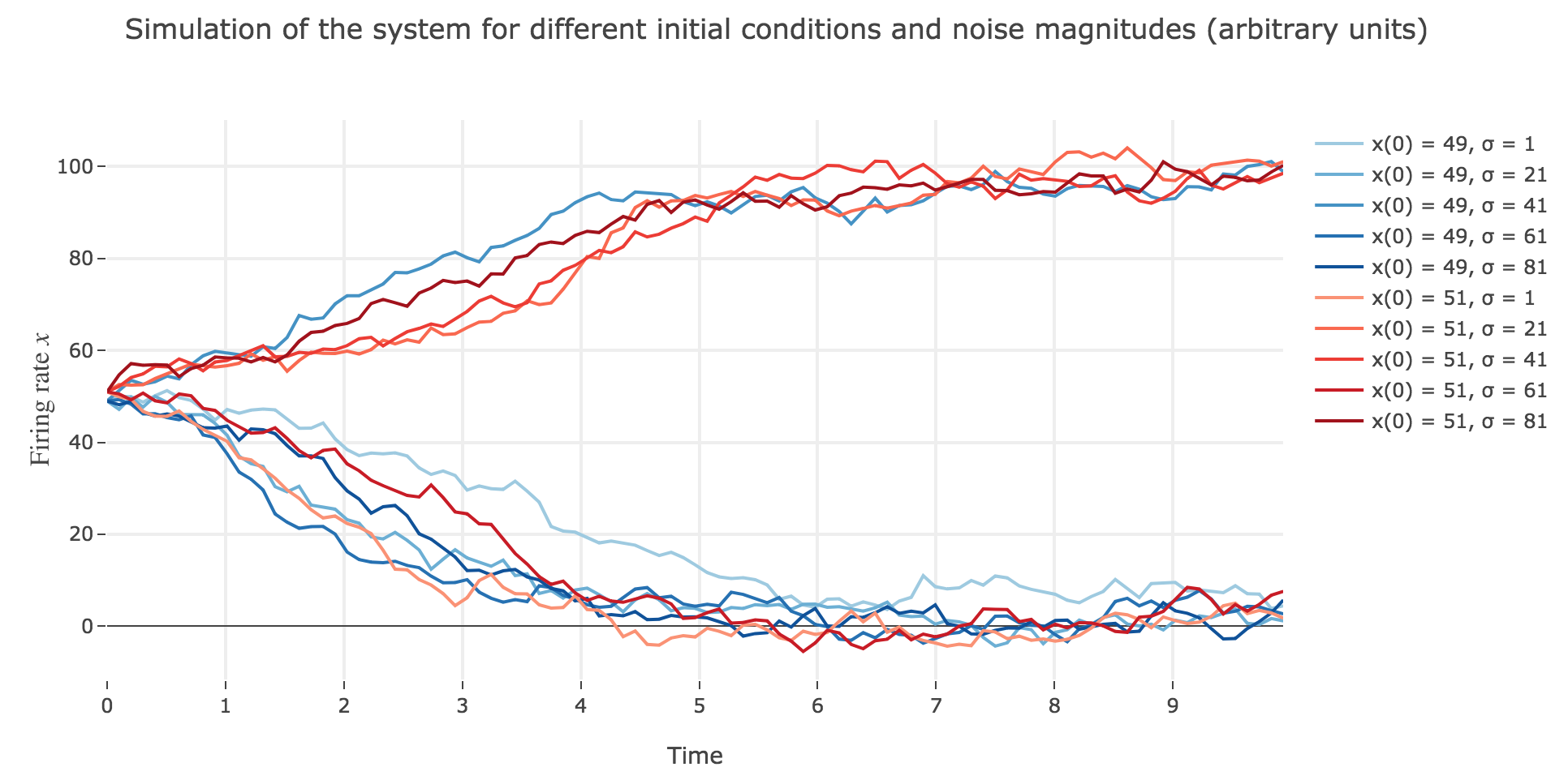
What appears in the above figures is that the bigger the noise magnitude $σ$ is, the more $x(t)$ is likely not to converge toward the expected stable fixed point (i.e. $98$ for $x>50$, $2$ for $x<50$).
This can be accounted for by the fact that the fixed points of dynamics change all the more that the noise magnitude is larger and larger: indeed, the larger the noise magnitude, the more the derivative $\dot{x}$ is modified (as the noise is added to it) and the more it moves away from its original value: new zero-crossings (i.e. fixed points) appear, other disappear, etc…:
To back this up: here is the evolution of the fixed points of the dynamics for different noise magnitudes (and different random seeds):
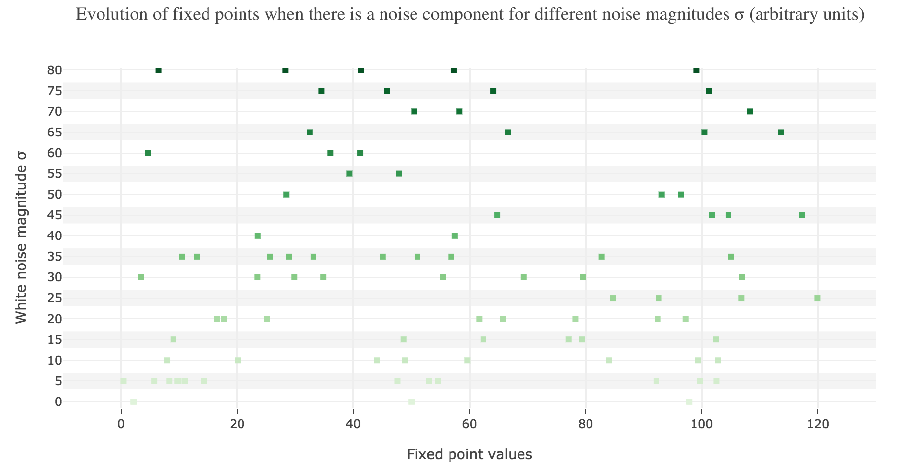
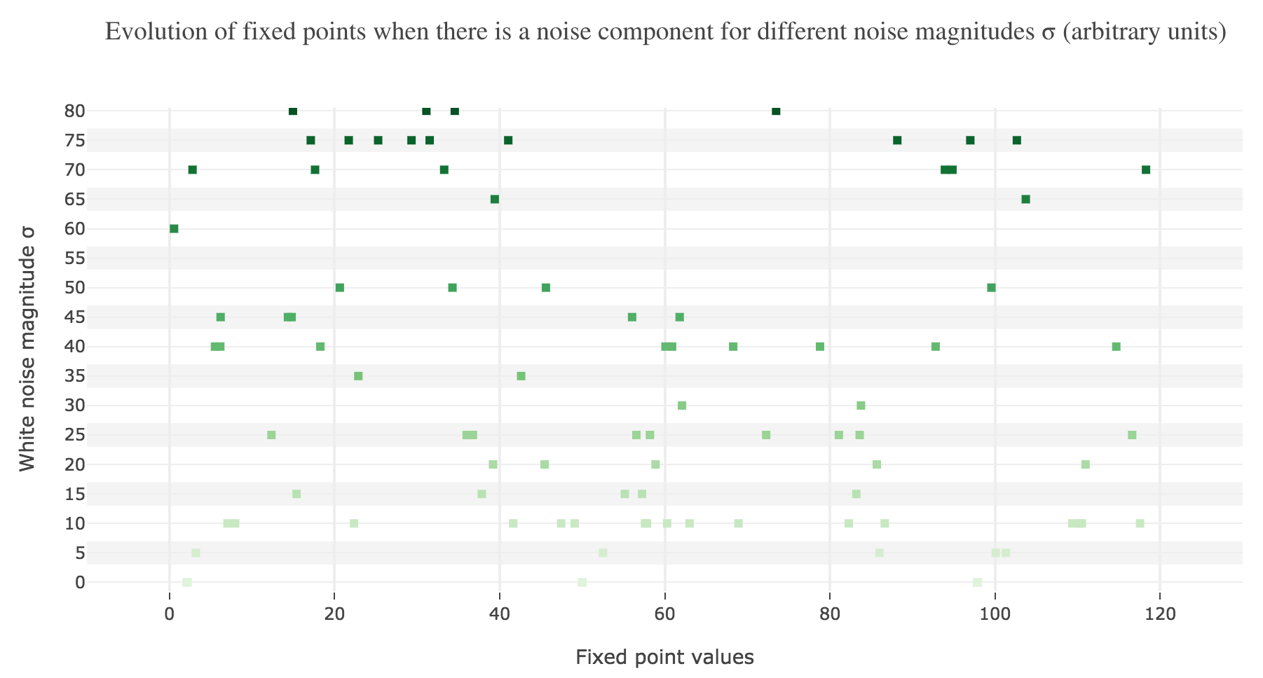
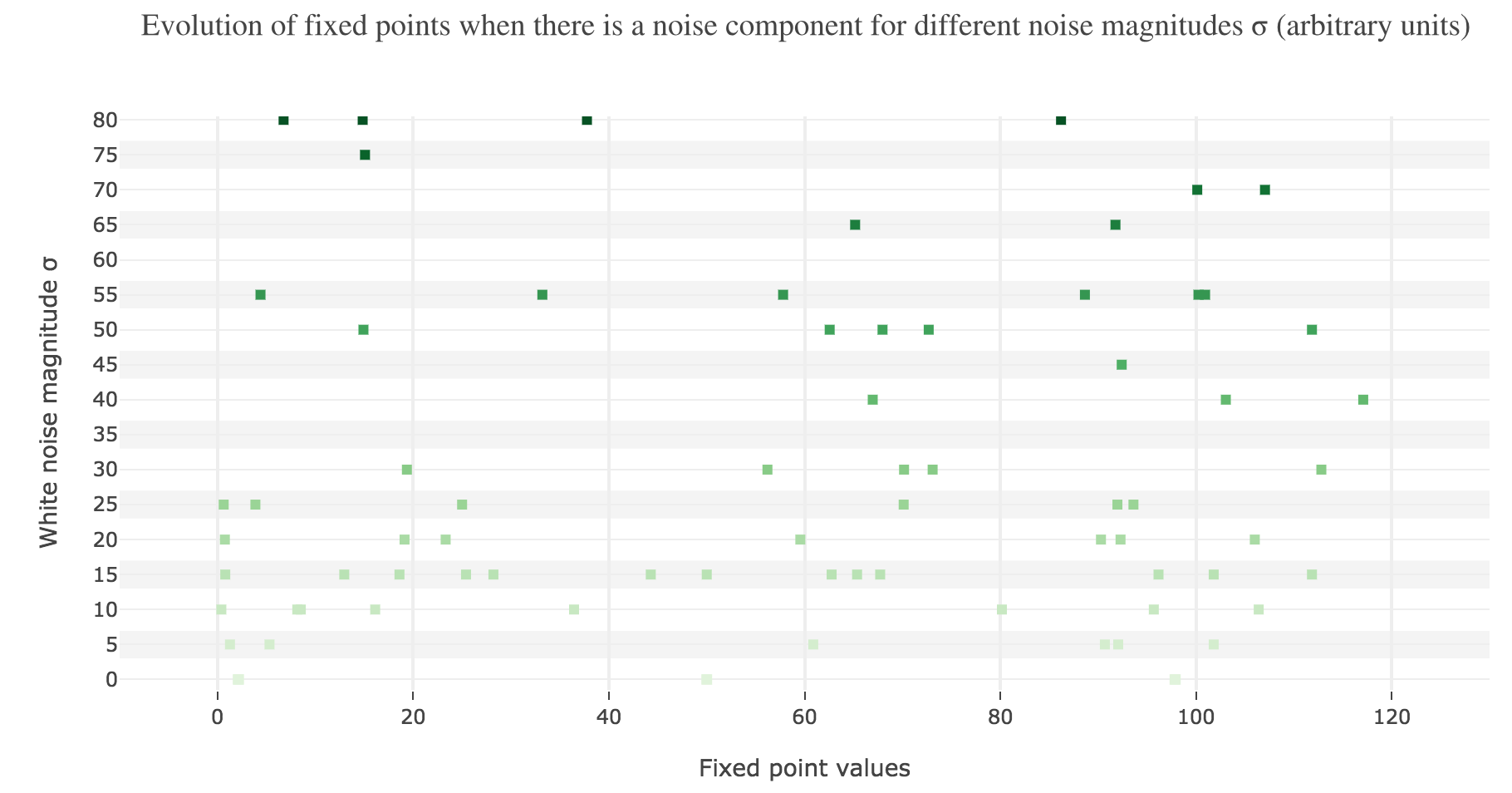
So the larger the noise magnitude, the “more” the set of fixed points is modified, resulting in $x(t)$ being less and less likely to converge toward the expected stable fixed point ($98$ for $x>50$, $2$ for $x<50$).
PROBLEM 2: Circuit with mutual inhibition
Link of the iPython notebook for the code
Now, let us consider a two-neurons circuit in which the neurons mutually inhibit one another. We will denote by
- $x_1$ and $x_2$ the firing rates of the two neurons
- $w = -0.1$ the inhibitory synaptic weight
- $I = 5$ an excitatory external input
- $f(s) ≝ 50 \, (1 + \tanh(s))$ the neurons’ activation function as before
1. Separate treatement of each neuron
We assume that we have the following differential equations:
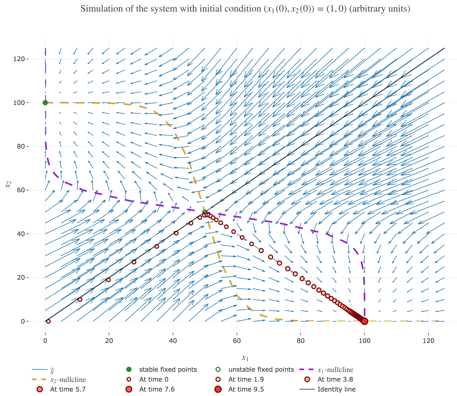
\[\begin{cases} \dot{x}_1(t) = -x_1(t) + f(w x_2(t) + I)\\ \dot{x}_2(t) = -x_2(t) + f(w x_1(t) + I)\\ \end{cases}\]which results in the following two-dimensional system dynamics flow:
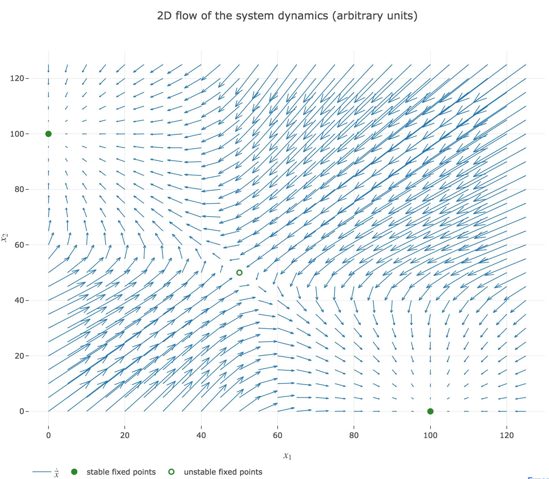
The nullclines of this system are the curves given by:
\[\begin{cases} \dot{x}_1(t) = 0 \\ \dot{x}_2(t) = 0 \end{cases}\]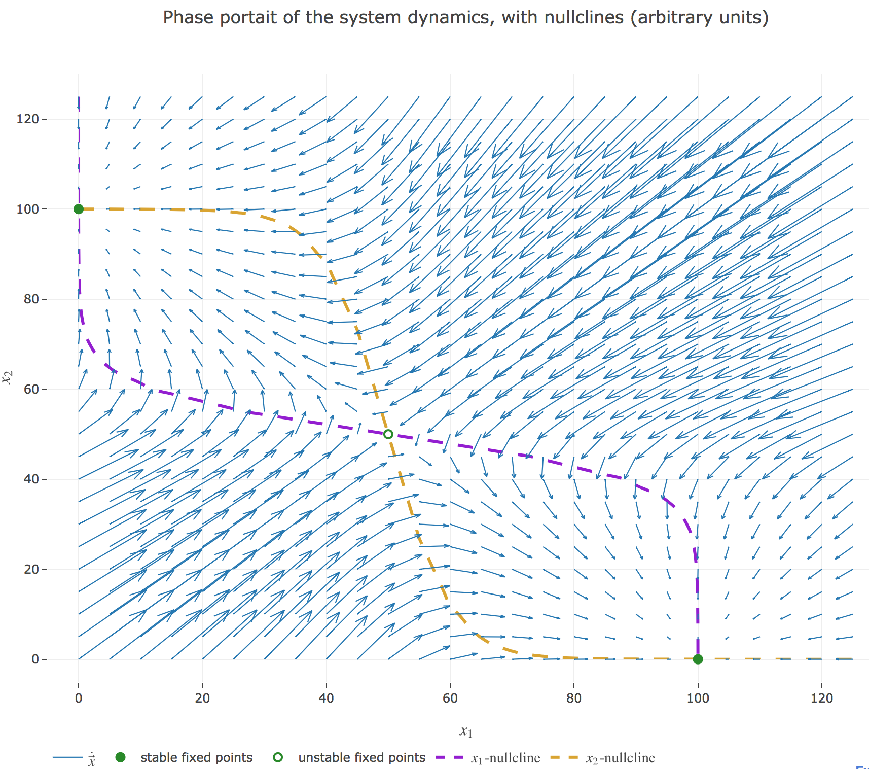
Their crossing points are the points at which both the $x_1$ derivative and the $x_2$ one vanish, i.e. the fixed points of the 2D-system dynamics. As before (cf. the previous problem), there are:
- stable fixed points: here, the points $(0, 100)$ and $(100, 0)$
- unstable fixed points: here, the point $(50, 50)$
We can easily check these are indeed fixed points of the dynamics:
-
For $(0, 100)$:
\[\begin{align*} -0+f(100w + I) &= f(-5) = 50(1+\tanh(-5))≃ 0 \\ -100+f(0w + I) &= f(5)-100 = 50(\underbrace{1+\tanh(5)}_{≃ 2}) - 100 ≃ 0 \end{align*}\]and it is symmetric for $(100, 0)$
-
For $(50, 50)$:
\[\begin{align*} -50+f(50w + I) &= f(0) - 50 = 50(1+\underbrace{\tanh(0)}_{=0}) - 50 = 0 \\ \end{align*}\]
System simulation
We set (arbitrary units):
- the time-increment to integrate the differential equation with the Euler method: $dt = Δt ≝ 0.1$
- The total duration $T = 10 = 100 Δt$
so that the Euler method yields, for $i ≠ j ∈ \lbrace 1, 2 \rbrace$:
\[\begin{align*} \quad & \frac{x_i(t+Δt) - x_i(t)}{Δt} = - x_i(t) + f\big(wx_j(t) + I\big) \\ ⟺ \quad & x_i(t+Δt) - x_i(t) = - x_i(t) Δt + f\big(wx_j(t) + I\big) Δt \\ ⟺ \quad & x_i(t+Δt) = (1 - Δt) x_i(t) + f\big(wx_j(t) + I\big) Δt \end{align*}\]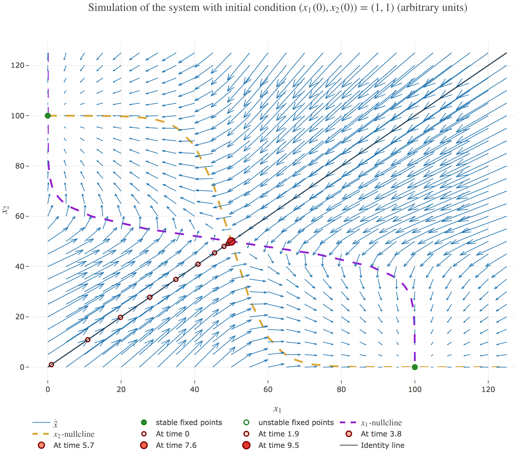
It appears that:
-
if $(x_1(0), x_2(0))$ is on the identity line – i.e. if $x_1(0) = x_2(0)$) – : $(x_1(t), x_2(t))$ converges toward the $(50, 50)$ unstable fixed point, as exemplified by figure 1.b.1.
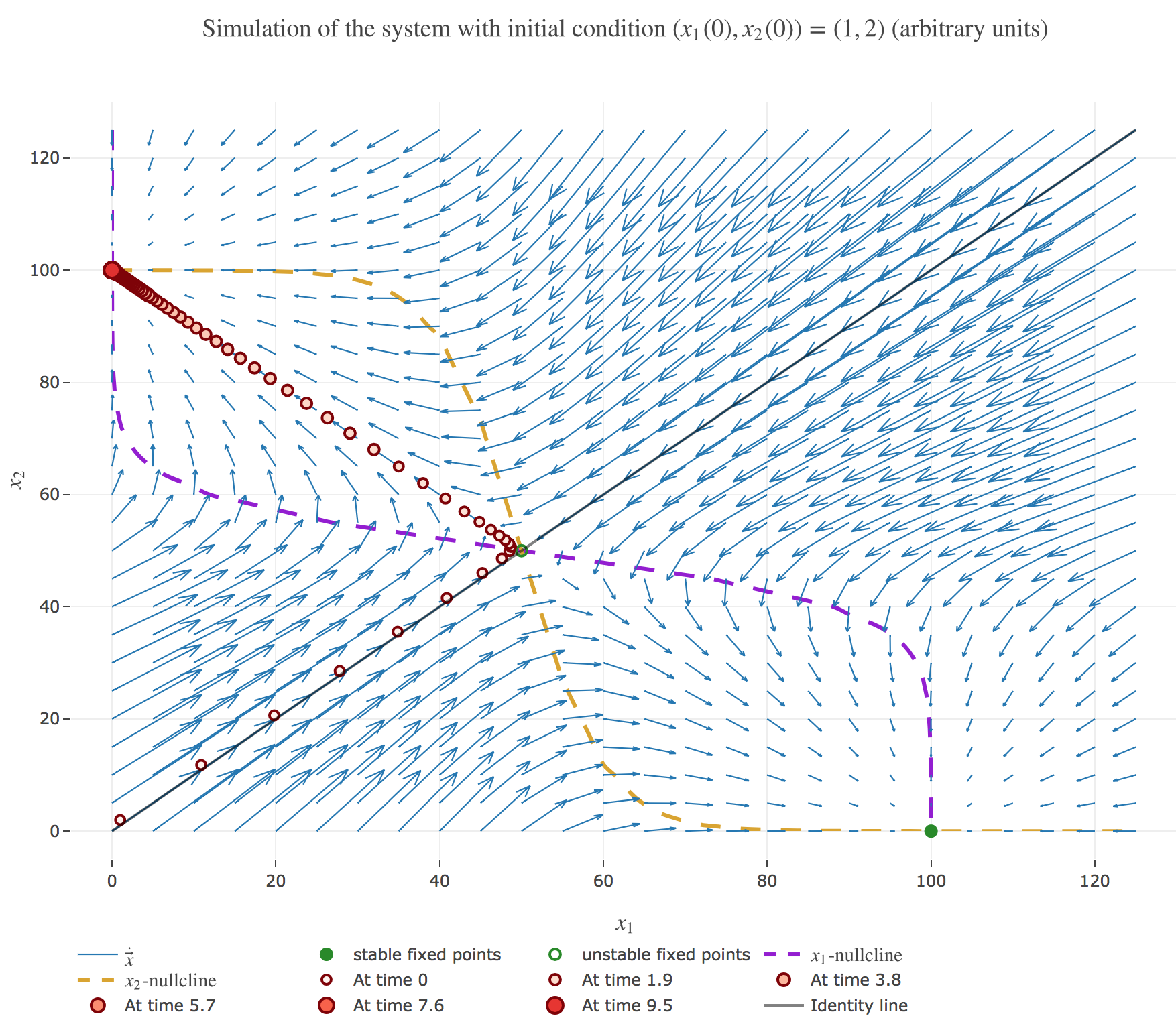
-
if $(x_1(0), x_2(0))$ is strictly above the identity line – i.e. if $x_1(0) < x_2(0)$) – : $(x_1(t), x_2(t))$ converges toward the $(0, 100)$ stable fixed point, as exemplified by figure 1.b.2.
-
if $(x_1(0), x_2(0))$ is strictly below the identity line – i.e. if $x_1(0) > x_2(0)$) – : $(x_1(t), x_2(t))$ converges toward the $(100, 0)$ stable fixed point, as exemplified by figure 1.b.3.
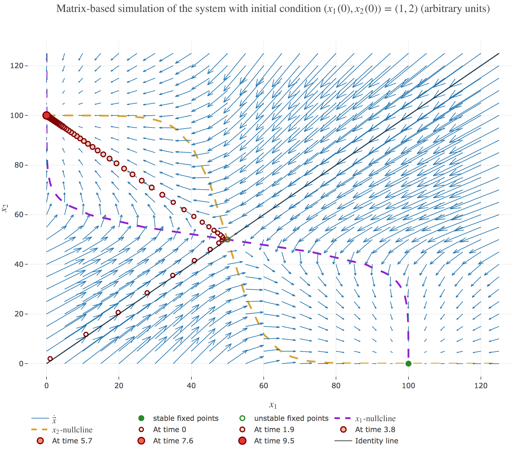
2. Vectorized system dynamics
We have hitherto treated each neuron separately, but there is a way to reduce the two differential equations to a single vectorized one:
\[\dot{\textbf{x}}(t) = - \textbf{x}(t) + f(W \textbf{x}(t) + \textbf{I})\]by setting:
- \[\textbf{x}(t) ≝ \begin{pmatrix} x_1(t)\\ x_2(t)\end{pmatrix} ∈ 𝔐_{2,1}(ℝ)\]
- \[W ≝ \begin{pmatrix} 0 & w\\ w & 0\end{pmatrix} ∈ 𝔐_2(ℝ)\]
- \[I ≝ \begin{pmatrix} I\\ I\end{pmatrix} ∈ 𝔐_{2,1}(ℝ)\]
as a result of which the Euler method gives:
\[\begin{align*} \quad & \frac 1 {Δt}\Big(\textbf{x}(t+Δt) - \textbf{x}(t)\Big) = - \textbf{x}(t) + f(W \textbf{x}(t) + \textbf{I}) \\ ⟺ \quad & \textbf{x}(t+Δt) = (1 - Δt)\, \textbf{x}(t) + Δt \, f(W \textbf{x}(t) + \textbf{I}) \end{align*}\]And we get the same simulations as before, for example with the initial condition $(x_1(0), x_2(0)) ≝ (1, 2)$:
PROBLEM 3: Hopfield Model
Link of the iPython notebook for the code
\[\newcommand{\T}{ {\raise{0.7ex}{\intercal}}} \newcommand{\sign}{\textrm{sign}}\]We will study the properties of a Hopfield network with $N = 64$ neurons, whose dynamics obeys the following differential equation:
\[\dot{\textbf{x}} = - \textbf{x} + f(W \textbf{x}) + σ η(t)\]where
-
$\textbf{x}$ is the firing rates vector
-
$W$ is the $N × N$ weight matrix
-
$η(t)$ is a Gaussian noise of magnitude $σ = 0.1$
-
the activation function $f ≝ \sign$ for the sake of simplicity
1. Storing a pattern
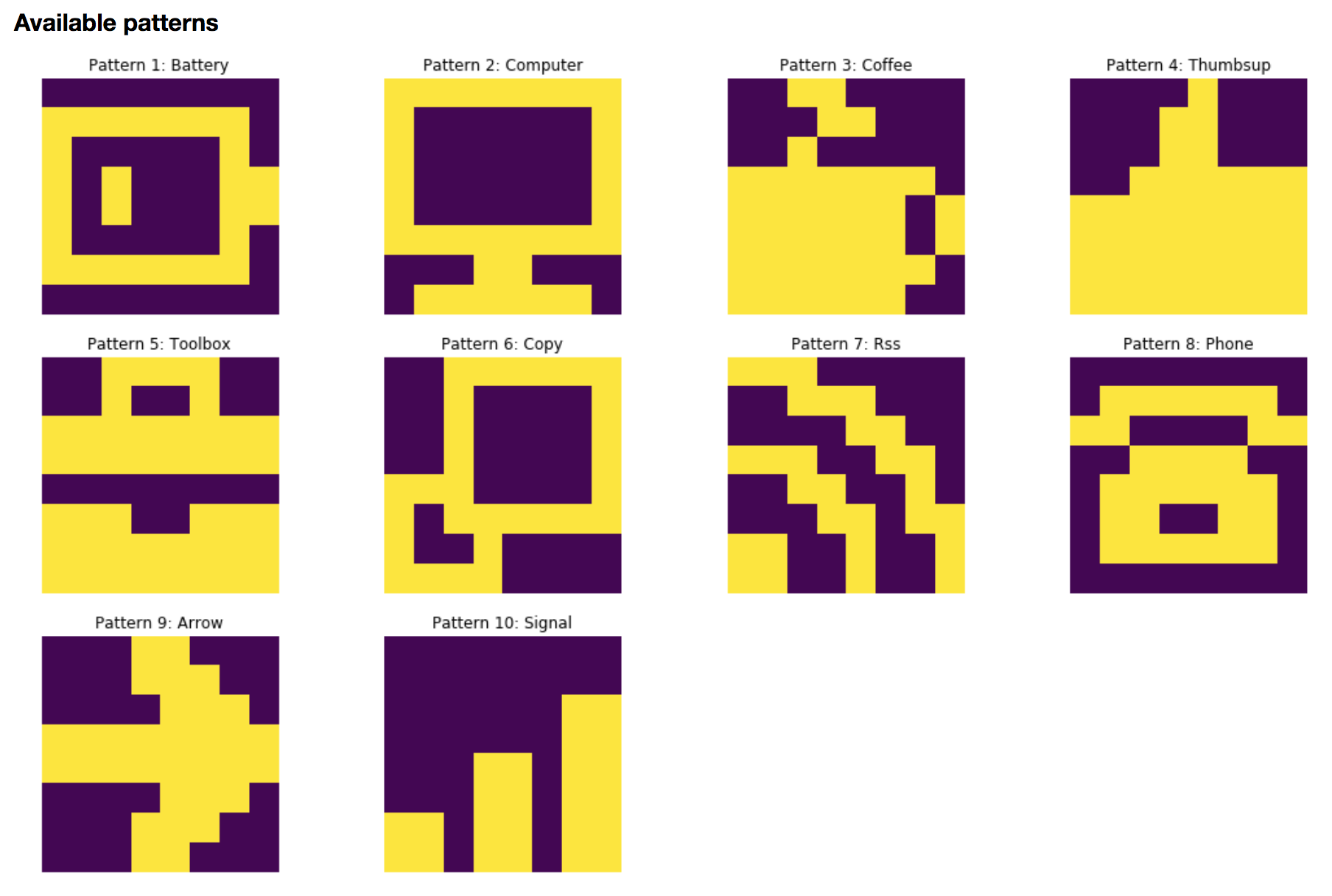
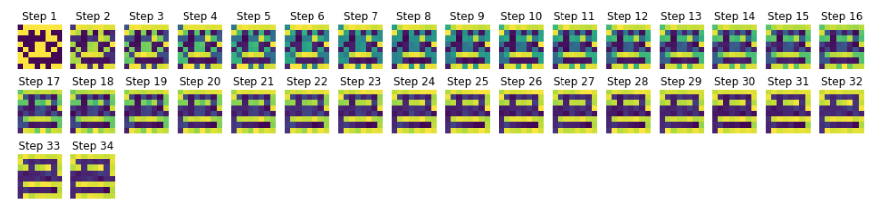
A pattern $\textbf{p} ∈ 𝔐_{N,1}(\lbrace -1, 1 \rbrace)$ is stored in the Hopfield network by setting:
\[W ≝ \frac 1 N \textbf{p} \textbf{p}^\T\]Here are some examples of patterns, visualized as $8×8$ images:
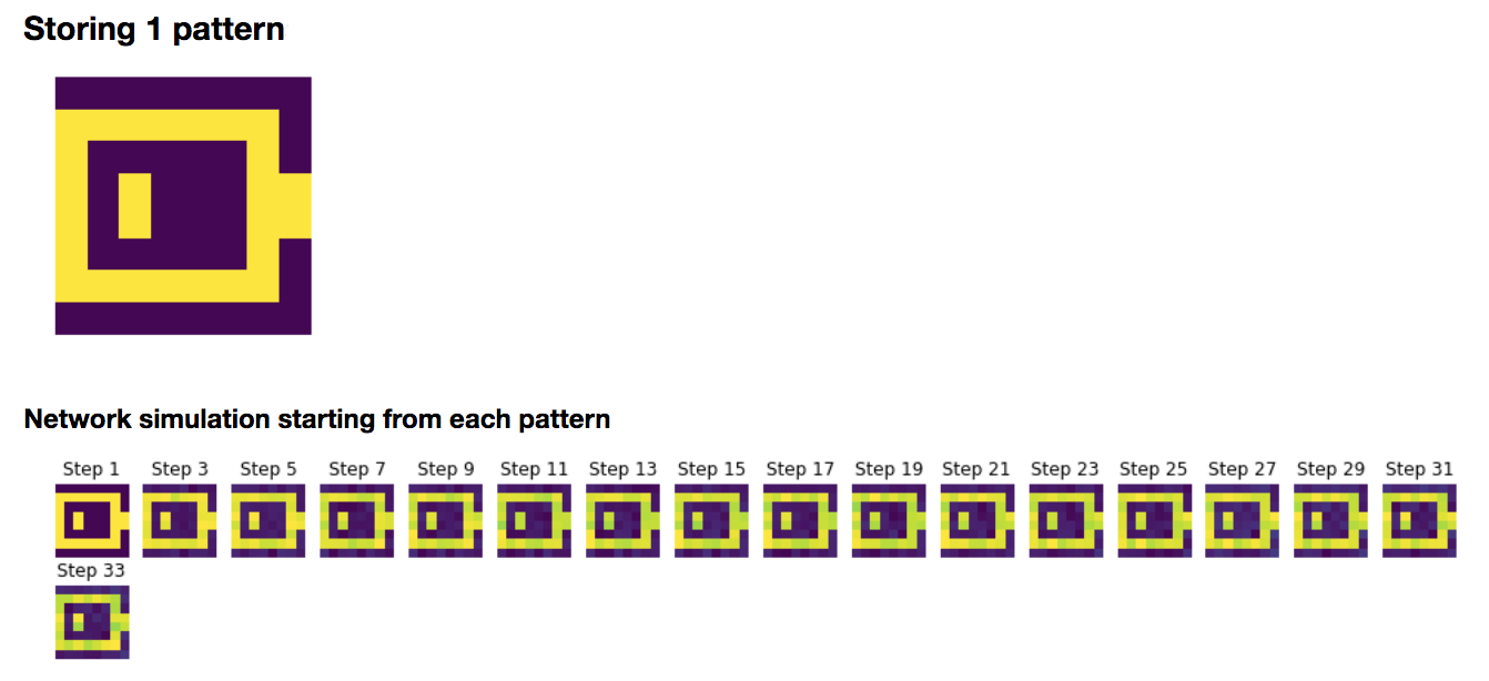
To begin with, let us focus on storing the battery pattern $\textbf{p}_{\text{bat}}$:

We set
\[W ≝ \frac 1 N \, \textbf{p}_{\text{bat}} \textbf{p}^\T_{\text{bat}}\]Then, we simulate the network with resort to the Euler method (with time-increment $dt = Δt ≝ 0.1$ (arbitrary units)):
\[\textbf{x}(t+Δt) = (1 - Δt)\, \textbf{x}(t) + Δt \, \sign(W \textbf{x}(t)) + \sqrt{Δt} \, σ η(t)\]which yields, for random starting patterns:
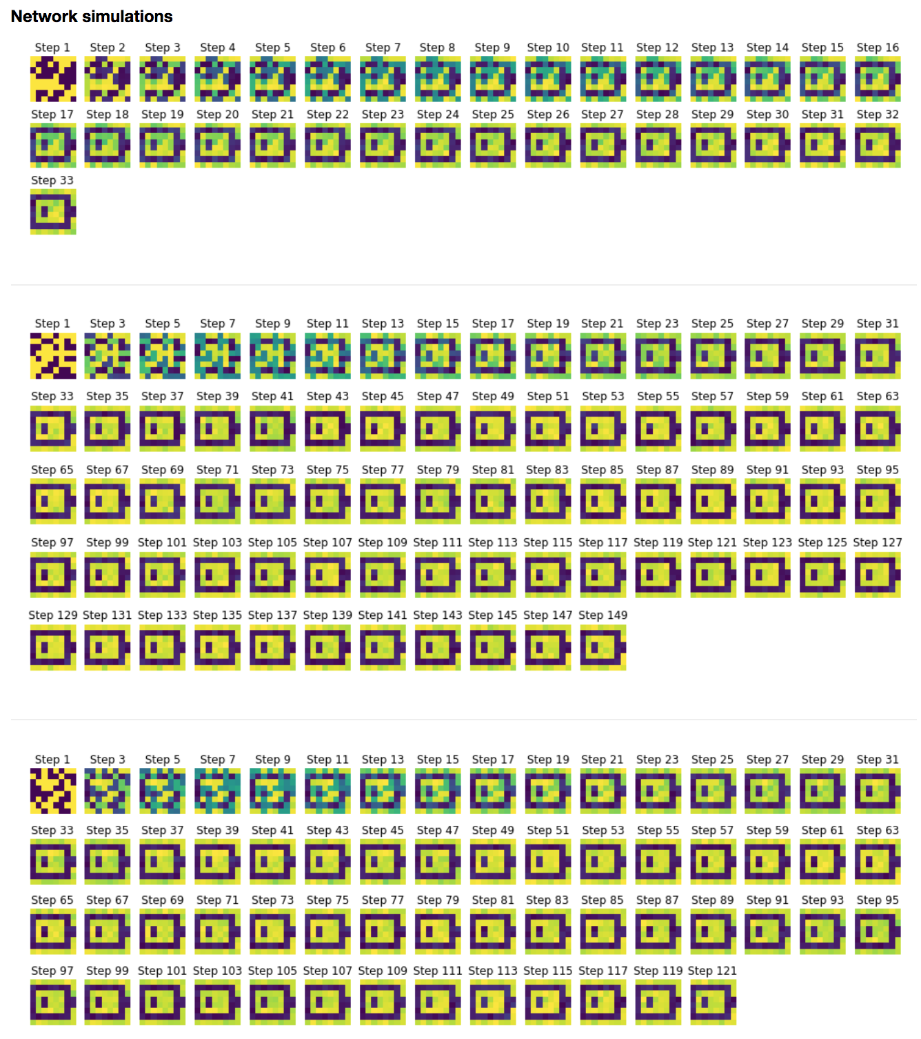

It can be noticed that the network relaxes to two fixed points, in our examples:
- the battery pattern: $\textbf{p}_{\text{bat}}$
- and its opposite pattern: $-\textbf{p}_{\text{bat}}$
From a theoretical standpoint, this can be explained by the fact that both $\textbf{p}{\text{bat}}$ and $-\textbf{p}{\text{bat}}$ are fixed points of the function
\[\textbf{x} ⟼ \sign(W\textbf{x})\]Indeed:
\[\begin{align*} \sign\left(W \textbf{p}_{\text{bat}}\right) & = \sign\left(\frac 1 N \left(\textbf{p}_{\text{bat}} {\textbf{p}_{\text{bat}}}^\T\right) \textbf{p}_{\text{bat}}\right) \\ & = \sign\left(\frac 1 N \textbf{p}_{\text{bat}} \left({\textbf{p}_{\text{bat}}}^\T \textbf{p}_{\text{bat}}\right)\right) &&\text{(because the matrix product is associative)}\\ &= \sign\Bigg(\frac 1 N \textbf{p}_{\text{bat}} \overbrace{\Bigg(\sum\limits_{ i=1 }^N \underbrace{ \left[\textbf{p}_{\text{bat}}\right]_i^2}_{= \; 1}\Bigg)}^{= \; N}\Bigg) \\ &= \sign\left(\textbf{p}_{\text{bat}}\right) \\ &= \textbf{p}_{\text{bat}} &&\text{(because } \textbf{p}_{\text{bat}} ∈ 𝔐_{N,1}(\lbrace -1, 1 \rbrace)\\ & &&\;\text{ so } \sign\left(\left[\textbf{p}_{\text{bat}}\right]_i\right) = \left[\textbf{p}_{\text{bat}}\right]_i \quad ∀1≤i≤N \text{ )} \end{align*}\]And:
\[\begin{align*} \sign\left(W (-\textbf{p}_{\text{bat}})\right) & = \sign\left(-W \textbf{p}_{\text{bat}}\right)\\ &= -\sign\left(W \textbf{p}_{\text{bat}}\right) &&\text{(because } \sign \text{ is an odd function)}\\ &= -\textbf{p}_{\text{bat}} \end{align*}\]Therefore, leaving the noise aside, by setting:
\[φ ≝ \textbf{x} ⟼ -\textbf{x} + \sign(W\textbf{x})\]so that the corresponding dynamics without noise is given by:
\[\dot{\textbf{x}} = φ(\textbf{x})\]it follows that:
\[φ(\textbf{p}_{\text{bat}}) = φ(-\textbf{p}_{\text{bat}}) = \textbf{0}\]As a result: $\textbf{p}{\text{bat}}$ and $-\textbf{p}{\text{bat}}$ are fixed points of the corresponding deterministic (i.e. without noise) dynamics, as a result of which the stochastic dynamics relaxes to them.
2. Storing two patterns
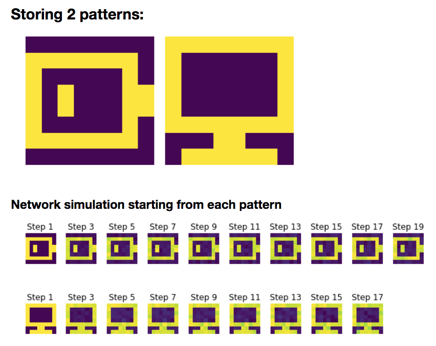
Now, let us add a new pattern $\textbf{p}_{\text{com}}$:
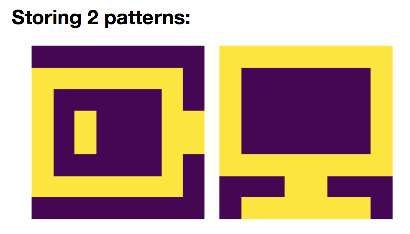
so that
\[W = \frac 1 N \left(\textbf{p}_{\text{bat}}\textbf{p}_{\text{bat}}^\T + \textbf{p}_{\text{com}}\textbf{p}_{\text{com}}^\T\right)\]And we simulate the network on random starting patterns:
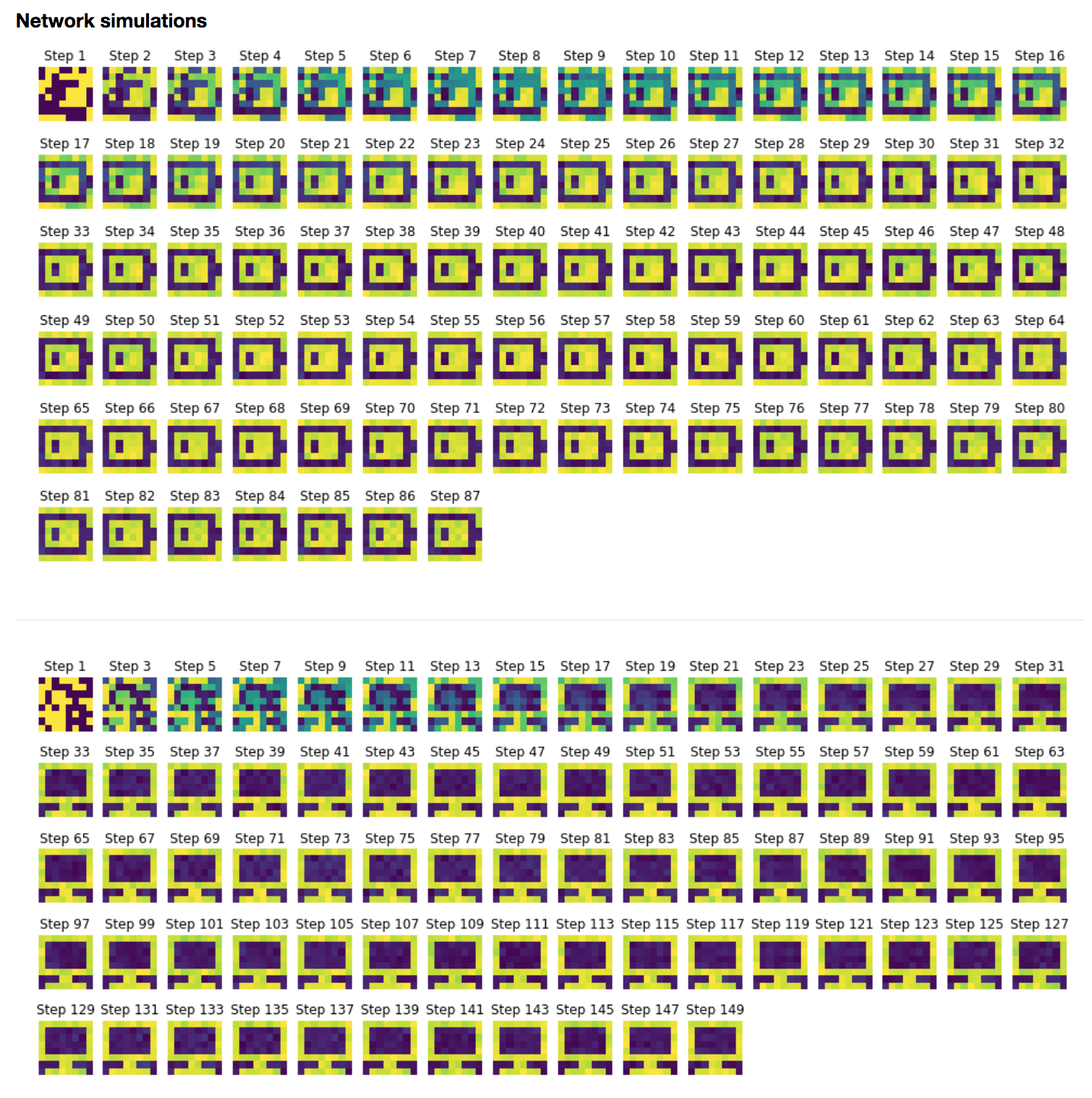
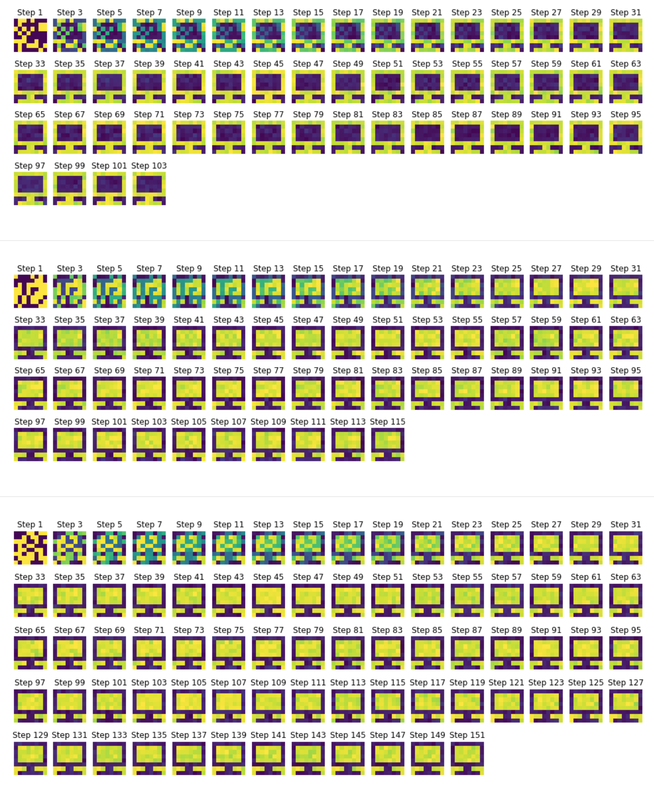
Again, we can show that:
- the battery pattern $\textbf{p}{\text{bat}}$ and its opposite pattern: $-\textbf{p}{\text{bat}}$
- the computer pattern $\textbf{p}{\text{com}}$ and its opposite pattern: $-\textbf{p}{\text{com}}$
are stored, owing to the fact that they are fixed points of the corresponding deterministic dynamics.
Indeed (for the sake of convenience, we set $\textbf{p} ≝ \textbf{p}{\text{bat}}$ and $\textbf{q} ≝ \textbf{p}{\text{com}}$):
\[\begin{align*} \sign\left(W \textbf{p}\right) & = \sign\left(\frac 1 N \left(\textbf{p} \textbf{p}^\T + \textbf{q} \textbf{q}^\T\right) \textbf{p}\right) \\ & = \sign\Big(\underbrace{\frac 1 N \left(\textbf{p} \textbf{p}^\T\right) \textbf{p}}_{\rlap{= \; \textbf{p} \; \text{(cf. previously)}}} + \frac 1 N \left(\textbf{q} \textbf{q}^\T\right) \textbf{p}\Big)\\ & = \sign\Big(\textbf{p} + \frac 1 N \, \textbf{q} \underbrace{\left(\textbf{q}^\T \textbf{p}\right)}_{\rlap{= \; ⟨\textbf{q},\, \textbf{p}⟩}}\Big)\\ \end{align*}\]But:
\[\vert ⟨\textbf{q},\, \textbf{p}⟩ \vert \, = \, \Bigg\vert \sum\limits_{ i = 1}^N \underbrace{[\textbf{q}]_i [\textbf{p}]_i}_{∈ \lbrace -1, 1 \rbrace} \Bigg\vert \, ≤ \, N\]And for $ε ∈ \lbrace -1, 1 \rbrace$:
\[\begin{align*} & ⟨\textbf{q},\, \textbf{p}⟩ = ε N \\ ⟺ \quad & \sum\limits_{ i = 1}^N [\textbf{q}]_i [\textbf{p}]_i = εN \\ ⟺ \quad & \sum\limits_{ i = 1}^N \underbrace{([\textbf{q}]_i [\textbf{p}]_i - ε)}_{≤ 0 \text{ if } ε = 1 \text{ else } ≥ 0} = 0 \\ ⟺ \quad & ∀1 ≤ i ≤ N, \quad [\textbf{q}]_i [\textbf{p}]_i - ε = 0\\ ⟺ \quad & ∀1 ≤ i ≤ N, \quad [\textbf{q}]_i [\textbf{p}]_i = ε\\ ⟺ \quad & ∀1 ≤ i ≤ N, \quad [\textbf{q}]_i = ε/[\textbf{p}]_i = ε[\textbf{p}]_i &&\text{ (because } [\textbf{p}]_i ∈ \lbrace -1, 1 \text{ )} \rbrace\\ \end{align*}\]NB: alternatively, we could have used the Cauchy-Schwarz inequality:
\[\vert ⟨\textbf{q},\, \textbf{p}⟩ \vert ≤ \underbrace{\Vert \textbf{q} \Vert_2 \, \Vert \textbf{p} \Vert_2}_{= \sqrt{N}\sqrt{N} = N} \quad \text{ and } \quad \Big(\vert ⟨\textbf{q},\, \textbf{p}⟩ \vert = N ⟺ \textbf{q} = ± \textbf{p} \Big)\]Here, as:
\[\textbf{q} ≠ \textbf{p} \quad \text{ and } \quad \textbf{q} ≠ -\textbf{p}\]it comes that:
\[\vert ⟨\textbf{q},\, \textbf{p}⟩ \vert < N\]Hence:
\[\begin{align*} \sign\left(W \textbf{p}\right) & = \sign\Big(\textbf{p} + \underbrace{\frac{\overbrace{⟨\textbf{q},\, \textbf{p}⟩}^{\rlap{∈ [-(N-1)\,, \,N-1] \; }}}{N}}_{∈ \, ]-1, 1[} \; \textbf{q}\Big)\\ &\overset{⊛}{=} \sign\left(\textbf{p}\right) &&\text{(because each } \frac {⟨\textbf{q},\, \textbf{p}⟩} N \, [\textbf{q}]_i ∈ \left[-1 + \frac 1 N, \, 1-\frac 1 N \right]\\ & && \quad \text{: it can't change the sign of } [\textbf{p}]_i ∈ \lbrace -1, 1 \rbrace\text{ )} \\ &= \textbf{p} \end{align*}\]And likewise, by symmetry:
\[\sign\left(W \textbf{q}\right) = \textbf{q}\]Once we know that $\textbf{p}$ and $\textbf{q}$ are fixed points, the same holds true for their opposites, as $\sign$ is an odd function (the proof is the same as previously).
So $±\textbf{p}$ and $±\textbf{q}$ are all fixed points of the corresponding deterministic dynamics, as a result of which the stochastic dynamics relaxes to them.
NB: in the computations, the key point is the equality $⊛$, which stems from $\textbf{q}$ being different from $±\textbf{p}$ (by Cauchy-Schwarz).
On top of that, it can be noted that the network relaxes to the fixed-point pattern which is the closest to the starting pattern! For example, consider the second-to-last and the third-to-last examples in figure 2.c.2:
- for both of these examples, in the starting pattern, we can distinguish what looks like the base of a (future) screen
- but the the second-to-last example converges to a bright-screen computer, whereas the third-to-last converges to a dark-screen one. This can be accounted for by the fact that there are more dark pixels in the third-to-last starting pattern than in the second-to-last one!
Therefore, we begin to see why Hopfield networks can be thought of as modeling an associative memory-like process: the starting patterns are similar to “visual clues”, to which the network associates the best (i.e. the closest) matching stored pattern.
3. The general rule
The general rule defining the weight matrix is:
\[W ≝ \frac 1 N \sum_{i=1}^M \textbf{p}_i \textbf{p}_i^\T\]where the $\textbf{p}_i$ are the patterns to be stored.
3 patterns: linear combinations stored
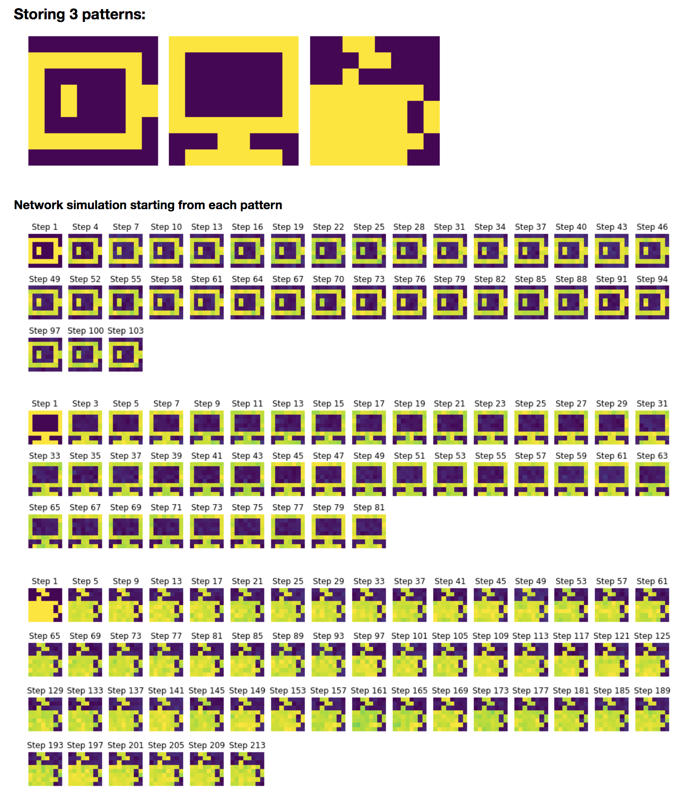
Let us add yet another pattern: $\textbf{p}_{\text{cof}}$:

so that, in compliance with the general rule:
\(W = \frac 1 N \left(\textbf{p}_{\text{bat}}\textbf{p}_{\text{bat}}^\T + \textbf{p}_{\text{com}}\textbf{p}_{\text{com}}^\T + \textbf{p}_{\text{cof}}\textbf{p}_{\text{cof}}^\T\right)\)
Then, we simulate the network with random initial conditions: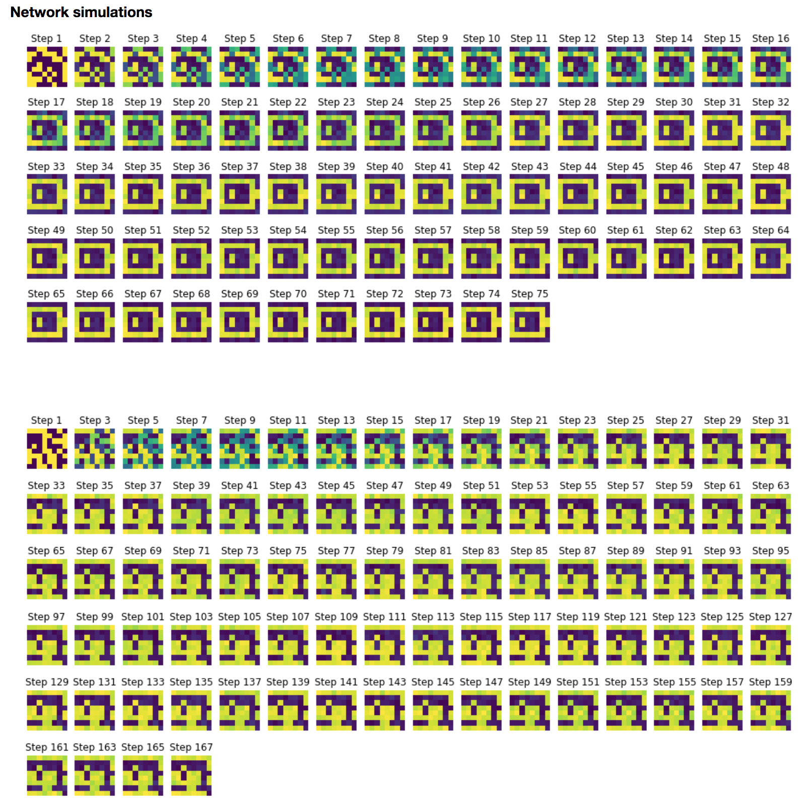

It appears that the networks relaxes to the following linear combinations of $\lbrace \textbf{p}_{\text{bat}}, \textbf{p}_{\text{com}}, \textbf{p}_{\text{cof}} \rbrace$ too:
- \[\textbf{p}_{\text{bat}} - \textbf{p}_{\text{com}} - \textbf{p}_{\text{cof}}\]
- \[\textbf{p}_{\text{bat}} - \textbf{p}_{\text{com}} + \textbf{p}_{\text{cof}}\]

So: on top of the patterns from which the weight matrix is constructed and their opposites, linear combinations thereof may also be stored.
Storing capacity
Finally, we will investigate how many patterns we can store in this $N=64$ neurons network by:
- adding new patterns, one after another
- and then simulating the network with each pattern as initial condition to see if the pattern is stored or not
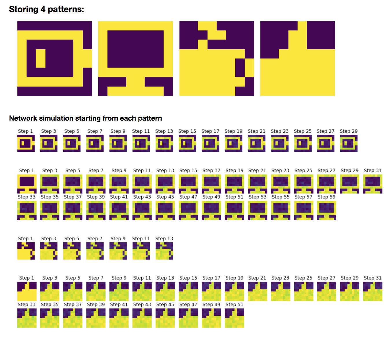
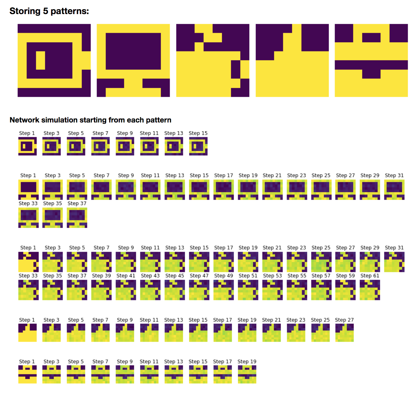
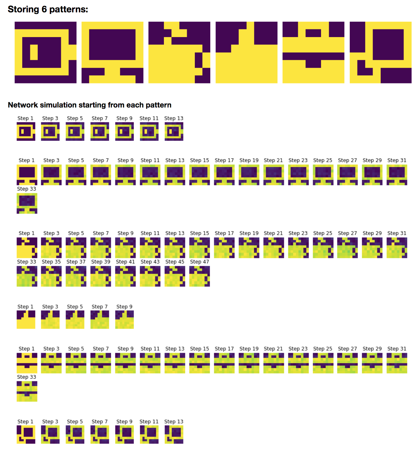
As a consequence:
- up until 6 (included) patterns: all the patterns are successfully stored
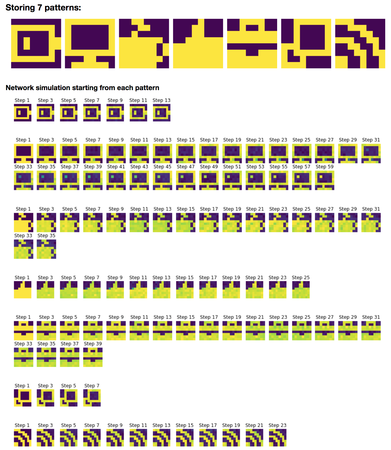
-
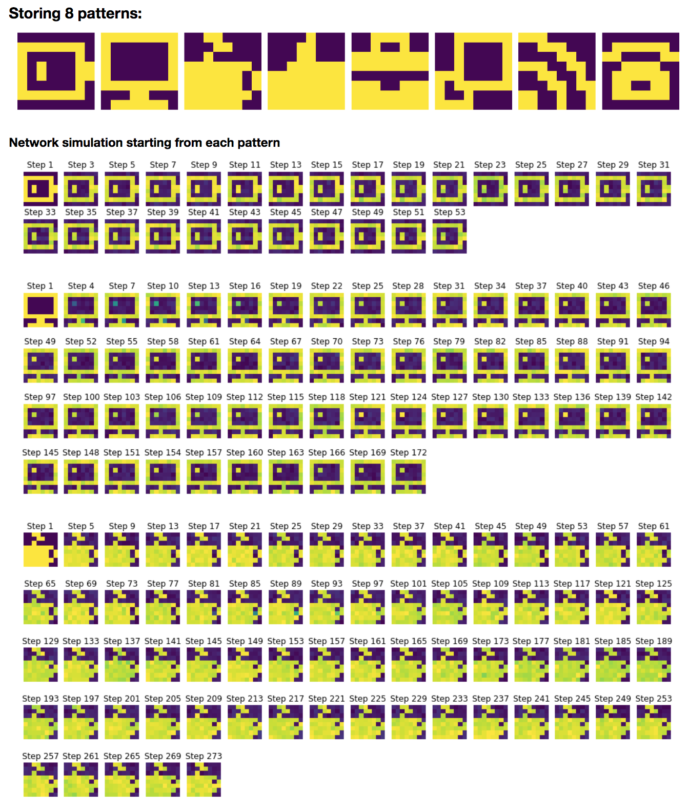
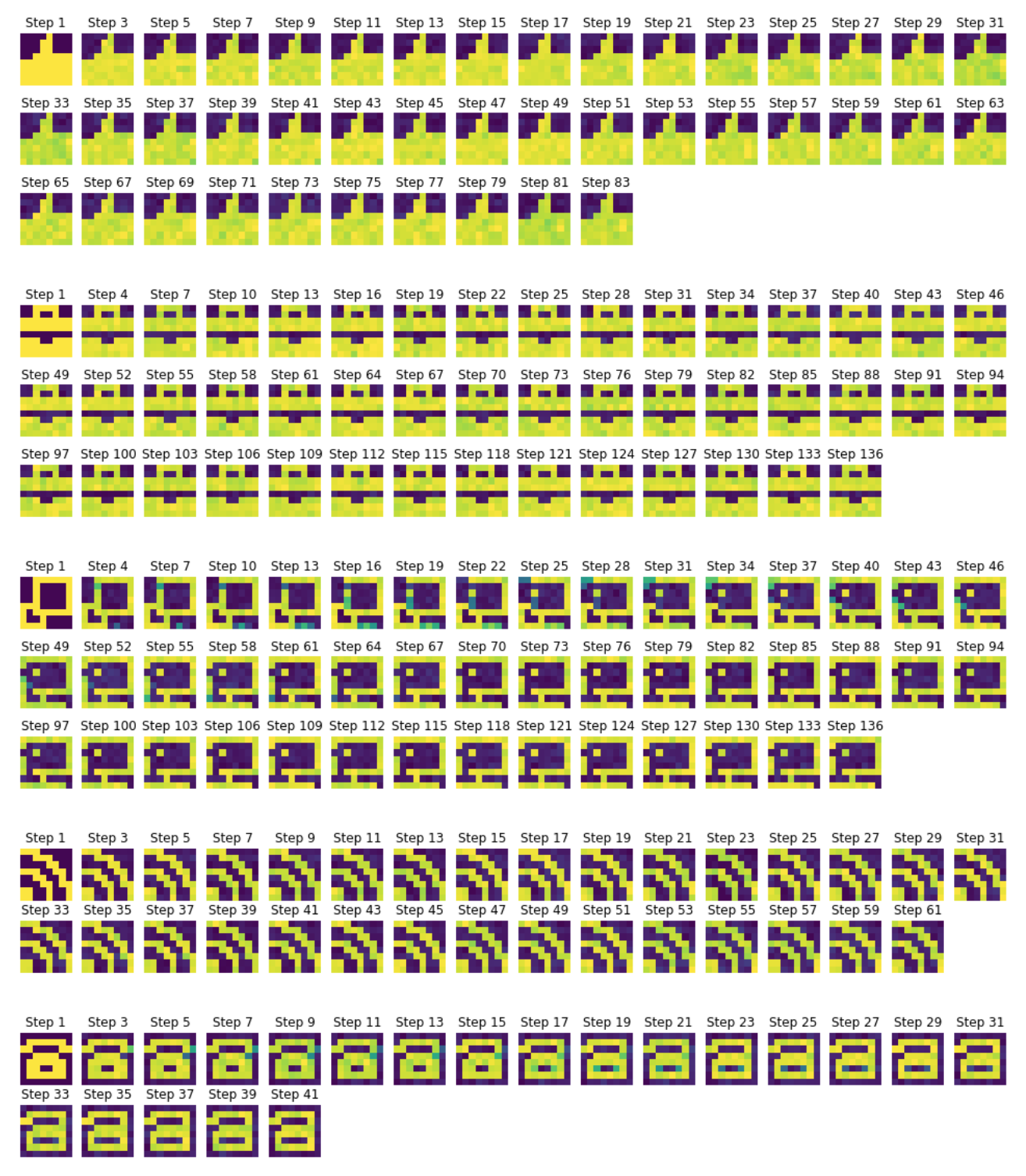
from 7 pattern on, some are not properly stored, and it gets worse and worse as the number of patterns increases:
- with 7 patterns: the computer screen is “prettified by bright pixels” (looking like light reflection!), but not stored unaltered
- with 8 patterns: on top of the light reflection on the computer screen, the copy icon is not stored at all: the network converges to an out-of-shape computer screen. In the same vein, the phone pattern ends up being deformed.
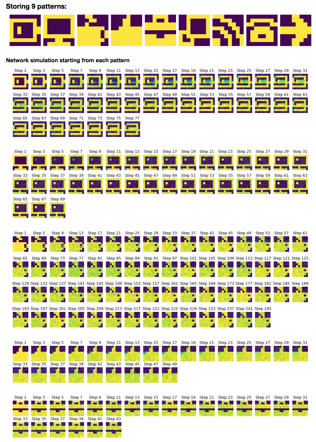
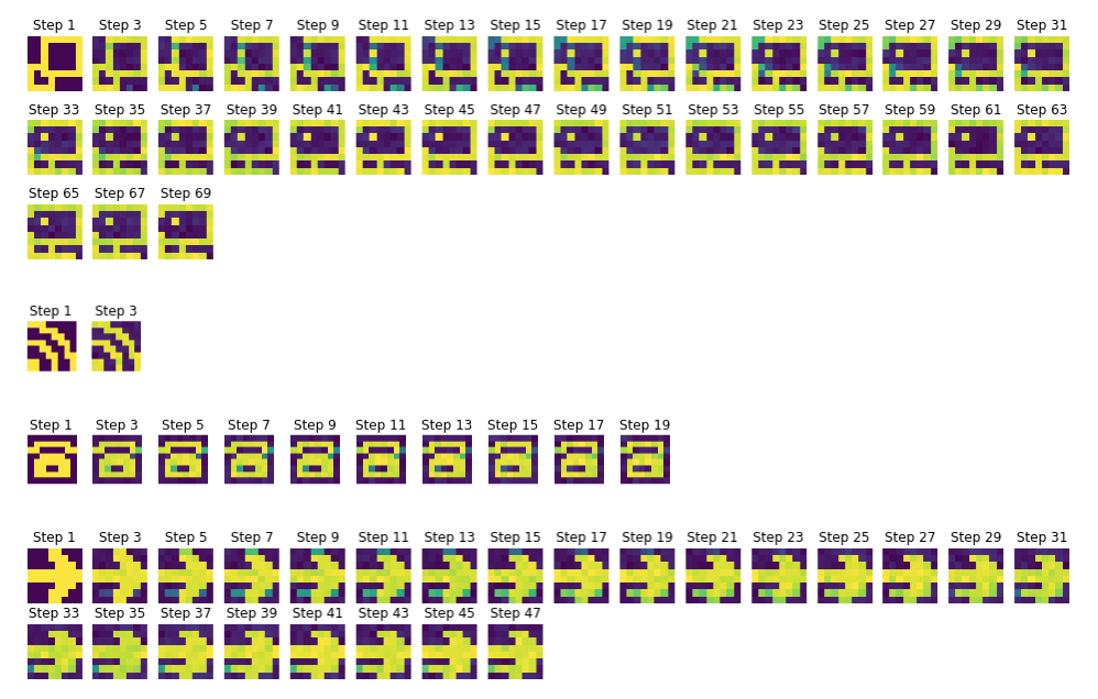
- with 9 patterns: the battery pattern is not stored anymore, the computer base is shifted, the cup of coffee, the thumbs up, the phone and the arrow are distorted, and the copy icon keeps converging toward the computer (they must look too similar for the full network’s pattern memory).
On the whole: the $64$-neurons Hopfield network can perfectly store $6$ patterns (and almost $7$ patterns, if it were not for the computer pattern ending up with a few bright pixels on the screen).
Leave a comment