Tutorial 4: Intent Recognition
Lab 4: Intent Recognition
Younesse Kaddar, Alexandre Olech and Kexin Ren (Lecturer: Mohamed Chetouani)
Exercice 1. Automatic detection of speaker’s intention from supra-segmental features
In this exercice, we consider a Human-Robot Interaction situation in which a human is evaluating actions performed by the Kismet robot: by showing approval or expressing prohibition. The initial corpus contains a total of 1002 American English utterances of varying linguistic content produced by three female speakers in three classes of affective communicative intents (aproval, attention, prohibition (weak)). The affective intents sound acted and are expressed rather strongly. The speech recordings are of variable length, mostly in the range of 1.8 - 3.25s. We extracted prosodic features such as the fundamental frequency (denoted by $f_0$ from now on) and energy. Files are respectively named *.f0 and *.en (and contain time, value entries on each line).
The aim of this exercice is to develop a human feedback classifier: positive (approval)/negative (prohibition). This classifier might be used to teach the robots and/or to guide the robot’s learning.
Development of the human feedback classifier:
- Extraction of prosodic features (f0 and energy)
- Extraction of functionals (statistics) that will be our features in the supervised learning task: mean, maximum, range, variance, median, first quartile, third quartile, mean absolute of local derivate
- Check functionals for both voiced (i.e. $f_0 ≠ 0$) and unvoiced segments, and then determine which segments are suited for the approach.
- Build two databases by randomly extracting examples: a learning database (60% of the data points) and a test one
- Train a classifer ($k$-nearest neighbors (k-NN) algorithm))
- Discuss the performance of the classifier
1. Extraction of prosodic features ($f_0$ and $energy$)
We found that, in the given data, the file names are contain either at, pw or ap, which are likely to represent the intention classes “Attention”, “Prohibition Weak” and “Approval” respectively.
Since the aim of this exercice is to develop a human feedback classifier for positive (“Approval”) / negative (“Prohibition”) intentions, we extract the files labelled as pw and ap and exclude the files labelled as at.
For our project, we cooperated online using Google Colab. The codes for extracting the files labelled as pw and ap and their the prosodic features is shown below:
import urllib.request
import numpy as np
import pandas as pd
from google.colab import files as google_files
import itertools
import matplotlib.pyplot as plt
import ggplot

def list_from_URL(file_URL, function_applied=None):
  lines_bytes = urllib.request.urlopen(file_URL).readlines()
  lines = []

  for line in lines_bytes:
    line = line.decode("utf-8").rstrip()

    if function_applied is not None:
      line = function_applied(line)

    lines.append(line)

  return lines

filenames = list_from_URL('https://raw.githubusercontent.com/youqad/Neurorobotics_Intent-Recognition/master/filenames.txt')
filenames = list(set(filenames))

files = []
indices = []

for file in filenames:

    URL_f0 = 'https://raw.githubusercontent.com/youqad/Neurorobotics_Intent-Recognition/master/data_files/{}.f0'.format(file)
    file_dicts = [{key:val for key, val in zip(['time', 'f0'], map(float, l.split()))} for l in list_from_URL(URL_f0)]

    URL_en = 'https://raw.githubusercontent.com/youqad/Neurorobotics_Intent-Recognition/master/data_files/{}.en'.format(file)
    for l, d in zip(list_from_URL(URL_en), file_dicts):
      d["file"] = file
      d["en"] = float(l.split()[1])
      d["label"] = file[-2:]

    files.extend(file_dicts)

# How `files` looks like:
# # files = [
# #           {"file": "cy0001at", "time": 0.02, "f0": 0., "en": 0.},
# #           {"file": "cy0001at", "time": 1.28, "f0": 0., "en": 0.},
# #           ...
# #           {"file": "li1450at", "time": 0.02, "f0": 0., "en": 0.},
# #           {"file": "li1450at", "time": 1.56, "f0": 404., "en": 65.}
# #         ]

pd.DataFrame(files).to_csv('data.csv', encoding='utf-8', index=False) # To reuse it next time
#google_files.download('data.csv')

# loading training data, once it has been saved on the repository
df = pd.read_csv('https://raw.githubusercontent.com/youqad/Neurorobotics_Intent-Recognition/master/data.csv').set_index('file')
df1 = df.loc[df['label'] != 'at']
2. Extraction of functionals (statistics) : mean, maximum, range, variance, median, first quartile, third quartile, mean absolute of local derivate
We calculated the mean, max, range, variance, median. first quartile, third quartile and mean absolute of local derivate for each en and f0 file. Using a pandas DataFrame, the code to extract these functionals is the following:
list_features  = ['mean',
                  'max',
                  ('range', lambda x: max(x)-min(x)),
                  'var',
                  'median',
                  ('1st_quantile', lambda x: x.quantile(.25)),
                  ('3rd_quantile', lambda x: x.quantile(.75)),
                  ('mean_absolute_local_derivate', lambda x: abs(x.diff()).mean())
                 ]

df1.groupby('file')['f0','en'].agg(list_features).head()
Table $1$ and Table $2$ show the first five lines of the statistics functionals of f0 and en files respectively:
Table $1$: Statistics of f0 files (first $5$ lines)
file |
mean |
max |
range |
var |
median |
1st_quantile |
3rd_quantile |
mean_absolute_local_derivate |
|---|---|---|---|---|---|---|---|---|
| cy0007pw | 92.3 | 257.0 | 257.0 | 10372.5 | 0.0 | 0.0 | 189.5 | 13.7 |
| cy0008pw | 78.4 | 250.0 | 250.0 | 9930.1 | 0.0 | 0.0 | 192.0 | 26.4 |
| cy0009pw | 69.1 | 243.0 | 243.0 | 8927.2 | 0.0 | 0.0 | 182.3 | 12.9 |
| cy0010pw | 29.2 | 221.0 | 221.0 | 4696.2 | 0.0 | 0.0 | 0.0 | 15.27 |
| cy0011pw | 110.7 | 230.0 | 230.0 | 9290.4 | 172.0 | 0.0 | 192.5 | 7.5 |
Table $2$: Statistics of en files (first $5$ lines)
file |
mean |
max |
range |
var |
median |
1st_quantile |
3rd_quantile |
mean_absolute_local_derivate |
|---|---|---|---|---|---|---|---|---|
| cy0007pw | 52.3 | 71.0 | 71.0 | 228.5 | 52.0 | 41.0 | 66.0 | 2.9 |
| cy0008pw | 47.7 | 70.0 | 70.0 | 321.9 | 43.0 | 41.0 | 64.5 | 3.9 |
| cy0009pw | 49.5 | 74.0 | 74.0 | 260.8 | 42.0 | 40.8 | 66.0 | 3.5 |
| cy0010pw | 46.1 | 77.0 | 77.0 | 165.8 | 42.0 | 41.0 | 50.8 | 3.3 |
| cy0011pw | 53.7 | 71.0 | 71.0 | 258.1 | 62.0 | 41.3 | 66.0 | 2.3 |
3. Check functionals for both voiced (i.e. $f_0$ ≠ $0$) and unvoiced segments. Which segments are suited for the approach?
We extract voiced segments by only keeping the data whose $f_0$ value is not equal to $0$. The code for extracting voiced sections and calculating the statistics of them is:
voiced = df1.loc[df1['f0']!=0].groupby('file')['f0','en'].agg(list_features)
voiced.head() # to visualize the first rows of the dataframe
Similarly, we extract the unvoiced segments by looking for the data whose $f_0$ value equals $0$. The code is:
unvoiced = df1.loc[df1['f0']==0].groupby('file')['en'].agg(list_features)
unvoiced.head()
The first $5$ lines of statistics for voiced segments in f0 and en files are shown in Table $3$ and Table $4$ respectively:
Table $3$: Statistics of f0 files of voiced segments (first $5$ lines)
file |
mean |
max |
range |
var |
median |
1st_quantile |
3rd_quantile |
mean_absolute_local_derivate |
|---|---|---|---|---|---|---|---|---|
| cy0007pw | 200.3 | 257.0 | 90.0 | 675.9 | 191.0 | 182.5 | 213.0 | 5.9 |
| cy0008pw | 200.0 | 250.0 | 83.0 | 538.4 | 198.5 | 179.5 | 210.0 | 10.4 |
| cy0009pw | 194.4 | 243.0 | 77.0 | 446.9 | 190.0 | 180.0 | 209.0 | 7.2 |
| cy0010pw | 186.1 | 221.0 | 67.0 | 465.3 | 178.5 | 171.3 | 204.3 | 6.5 |
| cy0011pw | 191.9 | 230.0 | 66.0 | 314.8 | 190.0 | 179.0 | 204.0 | 4.1 |
Table $4$: Statistics of en files of voiced segments (first $5$ lines)
file |
mean |
max |
range |
var |
median |
1st_quantile |
3rd_quantile |
mean_absolute_local_derivate |
|---|---|---|---|---|---|---|---|---|
| cy0007pw | 65.9 | 71.0 | 16.0 | 17.8 | 66.0 | 63.5 | 70.0 | 1.7 |
| cy0008pw | 61.0 | 70.0 | 70.0 | 242.7 | 66.0 | 61.5 | 68.0 | 5.8 |
| cy0009pw | 67.3 | 74.0 | 20.0 | 17.9 | 68.0 | 66.0 | 70.0 | 2.9 |
| cy0010pw | 65.8 | 77.0 | 25.0 | 50.5 | 64.0 | 62.0 | 70.8 | 4.0 |
| cy0011pw | 65.3 | 71.0 | 19.0 | 14.7 | 65.0 | 63.0 | 68.0 | 0.9 |
The first $5$ lines of statistics of unvoiced segments for en files are shown in Table $5$:
Table $5$: Statistics of en files of unvoiced segments (first $5$ lines)
file |
mean |
max |
range |
var |
median |
1st_quantile |
3rd_quantile |
mean_absolute_local_derivate |
|---|---|---|---|---|---|---|---|---|
| cy0007pw | 40.7 | 58.0 | 58.0 | 113.6 | 41.0 | 40.5 | 43.5 | 3.7 |
| cy0008pw | 39.2 | 58.0 | 58.0 | 189.6 | 42.0 | 41.0 | 43.0 | 5.2 |
| cy0009pw | 39.6 | 56.0 | 56.0 | 119.6 | 41.0 | 40.0 | 42.0 | 3.6 |
| cy0010pw | 42.4 | 68.0 | 68.0 | 101.4 | 41.0 | 40.0 | 43.0 | 3.1 |
| cy0011pw | 37.8 | 51.0 | 51.0 | 150.9 | 41.0 | 40.0 | 42.0 | 4.1 |
To judge which segments are better for the approach, we should check how separable (with respect to the label ap or pw) the data is in each situation. We first look at the overall statistics of the two segments for the two classes “Approval” and “Prohibition Weak”. The results are shown in Table $6$:
Table $6$: Statistics of “Approval” (ap) and “Prohibition Weak” (pw) files for voiced and unvoiced segments
segments |
file |
class |
mean |
max |
range |
var |
median |
1st_quantile |
3rd_quantile |
mean_absolute_local_derivate |
|---|---|---|---|---|---|---|---|---|---|---|
| voiced | f0 | ap | 289.5 | 597.0 | 521.0 | 11013.0 | 272.0 | 199.0 | 370.5 | 24.9 |
| voiced | f0 | pw | 192.4 | 597.0 | 522.0 | 2702.1 | 191.0 | 170.0 | 218.0 | 14.4 |
| voiced | en | ap | 73.3 | 93.0 | 93.0 | 88.2 | 74.0 | 68.0 | 79.0 | 3.5 |
| voiced | en | pw | 71.6 | 91.0 | 91.0 | 84.7 | 72.0 | 65.0 | 79.0 | 3.0 |
| unvoiced | f0 | ap | 0.0 | 0.0 | 0.0 | 0.0 | 0.0 | 0.0 | 0.0 | 0.0 |
| unvoiced | f0 | pw | 0.0 | 0.0 | 0.0 | 0.0 | 0.0 | 0.0 | 0.0 | 0.0 |
| unvoiced | en | ap | 46.4 | 94.0 | 94.0 | 239.2 | 43.0 | 41.0 | 55.0 | 3.9 |
| unvoiced | en | pw | 47.6 | 91.0 | 91.0 | 231.1 | 47.0 | 40.0 | 58.0 | 3.5 |
Table $6$ shows that, in voiced segments, the statistics of $f_0$ seem different for ap and pw files:
- the
enfunctionals of voiced and unvoiced segments seem very close to one another between the two types of classes (apandpw) - and of course, the statistics of
f0files for unvoiced segments are all $0$.
Thus, so far from the results of Table 6, $f_0$ values of voiced segments seem a better measurement for the approach.
This intuition is backed up by what we do next: by plotting the mean absolute local of derivate as a function of the variance for each type (voiced and unvoiced) of segments, we see that the data points seem more separable (based on their class) in the voiced case than in the unvoiced one:

Figure 1 suggests that the approval and prohibition classes can be reasonably well separated using their $f_0$ variance and mean absolute local derivate for voiced segments, supporting our previous idea voiced segments can be a good measurement for classifying.
However, by doing the same for unvoiced segments, we see that the data is not as easily separable:

Figure 2 shows that the data points cannot be separated well with respect to their classes using the variance and mean absolute local derivate of energy for unvoiced segments.
So on the whole, by plotting our randomly selected data, we found that voiced segments seem better suited for the classification task at hand.
4. Build two databases by randomly extracting examples : Learning database ($60$%) and Test database
We randomly extract $60$% data from the original dataset to build the training set and the remaining data was used as the test set. The code for this procedure is provided below:
def train_test(df=df1, train_percentage=.6, seed=1):

  voiced = df.loc[df['f0']!=0].groupby('file')['f0','en'].agg(list_features)
  unvoiced = df.loc[df['f0']==0].groupby('file')['en'].agg(list_features)

  X, Y = {}, {}

  X['voiced'], Y['voiced'] = {}, {}
  X['unvoiced'], Y['unvoiced'] = {}, {}


  X['voiced']['all'] = np.array(df.groupby('file')['f0','en'].agg(list_features))
  Y['voiced']['all'] = np.array(df.loc[df['f0']!=0].groupby(['file']).min().label.values)

  X['unvoiced']['all'] = np.array(unvoiced)
  Y['unvoiced']['all'] = np.array(df.loc[df['f0']==0].groupby(['file']).min().label.values)

  np.random.seed(seed)

  for type in ['voiced', 'unvoiced']:
    n = len(X[type]['all'])
    ind_rand = np.random.randint(n, size=int(train_percentage*n)) # random indices
    train_mask = np.zeros(n, dtype=bool)
    train_mask[ind_rand] = True
    X[type]['train'], X[type]['test'] = X[type]['all'][train_mask],  X[type]['all'][~train_mask]
    Y[type]['train'], Y[type]['test'] = Y[type]['all'][train_mask],  Y[type]['all'][~train_mask]

  return X, Y

X1, Y1 = train_test()
5. Train a classifer (k-NN method)
We used two implementations of a k-NN classifier, used both on voiced and unvoiced data:
- Scikit Learn’s kNN classifier
- our own implementation
We first use Scikit Learn’s kNN classifier to have a firsthand idea about the classification results. The code for Scikit Learn’s kNN classifier (with $k=3$) is shown below:
# Scikit Learn's kNN classifier:
# Just to test, but we will implement it ourselves of course!
from sklearn.neighbors import KNeighborsClassifier
from sklearn.metrics import accuracy_score

def sklearn_knn(k, X, Y):
  for type in ['voiced', 'unvoiced']:
    kNN = KNeighborsClassifier(n_neighbors=k)
    kNN.fit(X[type]['train'], Y[type]['train'])

    print("Accuracy score for {}: {:.2f}".format(type, accuracy_score(Y[type]['test'], kNN.predict(X[type]['test']))))
sklearn_knn(3, X1, Y1)
The classification result of Scikit Learn’s kNN classifier indicates that:
- Accuracy score of voiced data = $0.91$
- Accuracy score of unvoiced data = $0.61$
We can see that the accuracy of voiced data is 91%, much higher than the accuracy of unvoiced data which is only 61% (which confirms our previous intuition).
Then, we implement our own algorithm that we apply for both voiced and unvoiced data using the following code:
# Our own implementation!
from scipy.spatial.distance import cdist
from sklearn.metrics import confusion_matrix
from collections import Counter

def kNN(k, X, Y, labels=["pw", "ap"]):
    # auxiliary function: label prediction (by majority vote)
    # based on the nearest neighbors
    def predicted_label(ind_neighbors):
        label_neighbors = tuple(Y['train'][ind_neighbors])
        return Counter(label_neighbors).most_common(1)[0][0]

    # Pairwise distances between test and train data points
    dist_matrix = cdist(X['test'], X['train'], 'euclidean')
    y_predicted = []

    for i in range(len(X['test'])):
        ind_k_smallest = np.argpartition(dist_matrix[i, :], k)[:k]
        y_predicted.append(predicted_label(ind_k_smallest))

    # Confusion matrix: C[i, j] is the number of observations
    # known to be in group i but predicted to be in group j
    return confusion_matrix(Y['test'], np.array(y_predicted), labels=labels)

plt.figure()
cm = kNN(3, X1['voiced'], Y1['voiced'])
plot_confusion_matrix(cm, classes=["pw", "ap"],
                      title='Confusion matrix, with normalization')
plt.show()

cm2 = kNN(3, X1['unvoiced'], Y1['unvoiced'])
plot_confusion_matrix(cm2, classes=["pw", "ap"],
                      title='Confusion matrix, with normalization')
plt.show()
The result of our implementation is shown in Figure 3 and Figure 4:
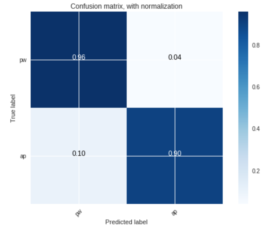
Figure 3 shows that, using voiced segments as training data, the accuracy of the classifier is very high:
- $92$% accuracy for the prohibition class
- and $91$% accuracy for the approval class
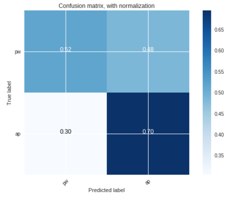
Figure 4 demonstrates that, using unvoiced segments as training data, the accuracy of the classifier is worse:
- ony $49$% for the prohibition class
- and $77$% for the approval class
The results above, again, support that voiced segments are better for training the classifier, and that they enable us to faithfully (with more than $90$% accuracy) separate the data points based their label, with $k=3$.
6. Evaluate and discuss the performance of the classifier. You will discuss the relevance of the parameters (f0 et energy), the role of the functionals, the role of $k$, ratio of Learning/Test databases, random design of databases.
Relevance of the parameters $f_0$ and energy
As shown in question 1.5, the classifier has relatively good results with voiced training data: more than $90$% of data points were correctly classified for each class. However, the results are more unsatisfactory with unvoiced training data: approximately $70$% of the approval data points and $50$% of the prohibition ones were correctly classified, which means that the recognition of prohibition data is more nettlesome than the recognition of approval data for unvoiced training data.
This better accuracy for voiced training data (which encompass the $f_0$ features, contrary to the unvoiced one), as well as the more separated data using $f_0$ shown in question 1.1.4, suggests that the $f_0$ parameter (the fundamental frequency) files may be more relevant/efficient than the energy to classify the sounds, provided that this fundamental frequency exists (which is the case for voiced sounds only).
Role of the functionals
We have plotted some $f_0$ functionals as a function of others. Figure 5 and Figure 6 show the $f_0$ mean absolute of local derivate, and variance as a function of the mean. We found that expressing the variance as a function of the mean led to a better separation of the data points. As such, that these functionals come really in handy when it comes to classifying the data points by the k-NN method.

Role of $k$
By implementing the k-NN classifier using different $k$ values, we found that with a higher $k$, the pw data can be classified more accurately, but the ap data will be classified less accurately. This may be due to larger values of $k$ reducing noise effect on the classification, but making boundaries between the classes less distinct.
Ratio of Learning/Testing data
By testing the accuracy of classifier with different ratio values, we found that the classifier becomes less accurate for lower values of the ratio (due to a lack of training) and for larger values of the ratio as well (due to overfitting of the data).
Exercice 2. Detection of multiple intents
1. Extract the prosodic features ($f_0$ and energy) and their functionals
Here, we use the same method than in question 1.1, using the pandas DataFrame df instead of df1:
df.groupby('file')['f0','en'].agg(list_features).head()
2. Develop a classifier for these three classses
We then develop a classifier which takes into account the third class (attention): this one corresponds to data points which are neither approvals nor prohibitions.
X, Y = train_test(df=df)
sklearn_knn(3, X, Y)
plt.figure()
cm = kNN(3, X['voiced'], Y['voiced'], labels=["pw", "ap", "at"])
plot_confusion_matrix(cm, classes=["pw", "ap", "at"],
                      title='Confusion matrix, with normalization')
plt.show()

cm2 = kNN(3, X['unvoiced'], Y['unvoiced'], labels=["pw", "ap", "at"])
plot_confusion_matrix(cm2, classes=["pw", "ap", "at"],
                      title='Confusion matrix, with normalization')
plt.show()
3. Evaluate and discuss the performance of the classifier. We could use confusion matrices.
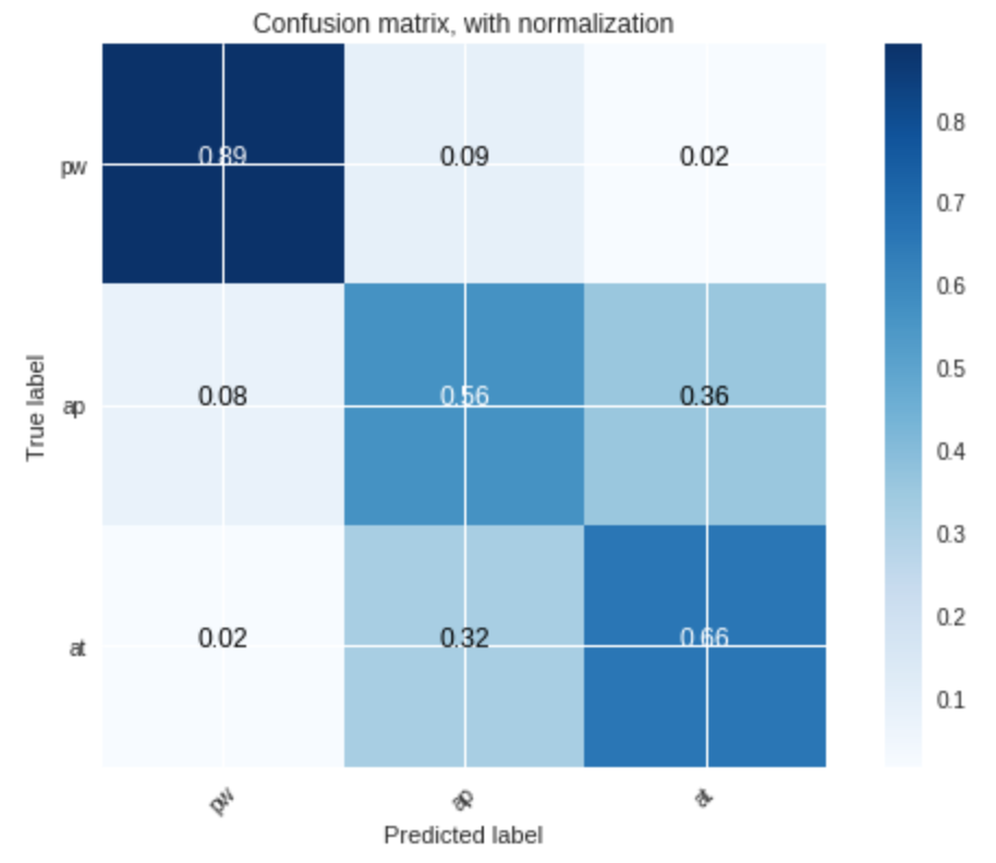
As before, the classifier is more accurate for voiced segments than for unvoiced ones:
-
for voiced segments:
- more than $80$% of the prohibition sounds
- $56$% of the approval ones
- and $66$% of the attention ones
were correctly classified.
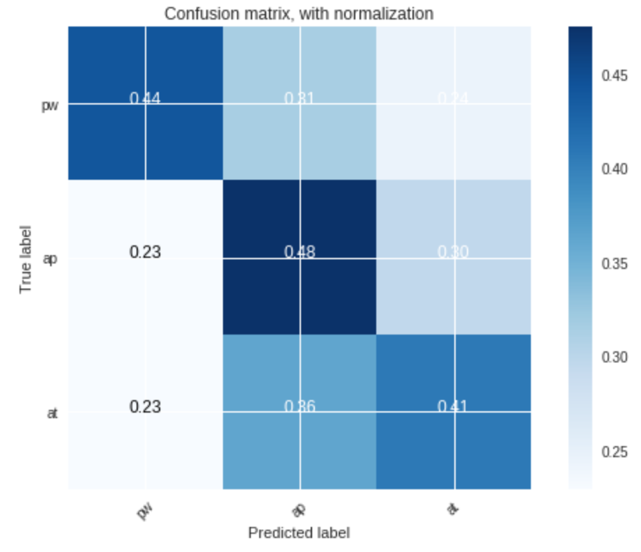
-
for unvoiced segments: the results are, as exepected, worse: only $51%$ of the prohibition, $45%$ of the approval and $37%$ of the attention sounds were correctly recognized.
On the whole:
- prohibition sounds are definitely the most recognizable ones, as indicated by the high corresponding accuracy rate
- however, the attention sounds seem to mess the approval class recognition up: the classifier has a harder time recognizing the approval sounds now that there are additional attention sounds. This has a rather intuitive explanation: one can conceive that it is easy to mistake an approval sentence with an attention-drawing one, as the tone of the voice generally rises in a similar fashion.
Leave a comment