Exercise Sheet 4: Covariance and Correlation, Bayes’ theorem, and Linear discriminant analysis
Exercise Sheet 4: Covariance and Correlation, Bayes’ theorem, and Linear discriminant analysis
Younesse Kaddar
\[\newcommand{\Var}{\mathop{\rm Var}\nolimits} \newcommand{\Cov}{\mathop{\rm Cov}\nolimits}\]1. Covariance and Correlation
Assume that we have recorded two neurons in the two-alternative-forced choice task discussed in class. We denote the firing rate of neuron $1$ in trial $i$ as $r_{1,i}$ and the firing rate of neuron $2$ as $r_{2,i}$. We furthermore denote the averaged firing rate of neuron $1$ as $\bar{r}_1$ and of neuron $2$ as $\bar{r}_2$. Let us “center” the data by defining two data vectors:
\[\textbf{x} ≝ \begin{pmatrix} r_{1, 1} - \bar{r}_1 \\ \vdots \\ r_{1, N} - \bar{r}_1 \\ \end{pmatrix} \qquad \textbf{y} ≝ \begin{pmatrix} r_{2, 1} - \bar{r}_2 \\ \vdots \\ r_{2, N} - \bar{r}_2 \\ \end{pmatrix}\](a) Show that the variance of the firing rates of the first neuron is:
\[\Var(r_1) = \frac{1}{N-1} \Vert x \Vert^2\]The actual variance of $r_1$ is not known. So to estimate it, we compute the average of the squared deviations on a sample ($r_{1, 1}, ⋯, r_{1, N}$) of the population: the biased sample variance:
\[\Var_{biased}(r_1) = \frac{1}{N} \sum\limits_{ i=1 }^N \big(r_{1, i} - \underbrace{\bar{r}_1}_{\rlap{= \frac 1 N \sum\limits_{i=1 }^N r_{1, i}}}\big)^2\]To what extent is this estimate biased? By denoting by $μ_1$ (resp. $\Var(r_1)$) the actual mean (resp. variance) of $r_1$:
\[\begin{align*} 𝔼(\Var_{biased}(r_1)) & = \frac 1 N \, 𝔼\left(\sum\limits_{ i=1 }^N \big(r_{1, i} - \bar{r}_1\big)^2\right) \\ & = \frac 1 N \, 𝔼\left(\sum\limits_{ i=1 }^N \left(r_{1, i} - \frac 1 N \sum\limits_{ j=1 }^N r_{1, j} \right)^2\right) \\ & = \frac 1 N \, 𝔼\left(\sum\limits_{ i=1 }^N r_{1, i}^2 - \frac 2 N r_{1, i} \sum\limits_{ j=1 }^N r_{1, j} + \frac 1 {N^2} \left(\sum\limits_{ j=1 }^N r_{1, j}\right)^2 \right) \\ & = \frac 1 N \, 𝔼\left(\sum\limits_{ i=1 }^N r_{1, i}^2 - \frac 2 N r_{1, i} \sum\limits_{ j=1 }^N r_{1, j} + \frac 1 {N^2} \sum\limits_{ 1 ≤ j, k ≤ N } r_{1, j} \; r_{1, k} \right) \\ & = \frac 1 N \, \left(\sum\limits_{ i=1 }^N 𝔼(r_{1, i}^2) - \frac 2 N \sum\limits_{ j=1 }^N 𝔼(r_{1, i}\; r_{1, j}) + \frac 1 {N^2} \sum\limits_{ 1 ≤ j, k ≤ N } 𝔼(r_{1, j} \; r_{1, k}) \right) \\ & = \frac 1 N \, \Bigg(\sum\limits_{ i=1 }^N 𝔼(r_{1, i}^2) - \frac 2 N 𝔼(r_{1, i}^2) - \frac 2 N \sum\limits_{ \substack{j=1\\ j≠i} }^N 𝔼(r_{1, i})\; 𝔼(r_{1, j})\\& \qquad \qquad + \frac 1 {N^2} \sum\limits_{ 1 ≤ j ≤ N } 𝔼(r_{1, j}^2) + \frac 1 {N^2} \sum\limits_{ 1 ≤ j ≠ k ≤ N } 𝔼(r_{1, j}) \; 𝔼(r_{1, k}) \Bigg) && \text{(by independence)}\\ &= \frac 1 N \, \Bigg(N \, 𝔼(r_{1, i}^2) - 2 \, 𝔼(r_{1, i}^2) - 2 \, \sum\limits_{ \substack{j=1\\ j≠i} }^N 𝔼(r_{1, i})\; 𝔼(r_{1, j})\\& \qquad \qquad + \frac 1 N \sum\limits_{ 1 ≤ j ≤ N } 𝔼(r_{1, j}^2) + \frac 1 N \sum\limits_{ 1 ≤ j ≠ k ≤ N } 𝔼(r_{1, j}) \; 𝔼(r_{1, k}) \Bigg)\\ &= \frac 1 N \, \Bigg(N \, \underbrace{𝔼(r_{1, i}^2)}_{≝ \; \Var(r_1) + μ_1^2} - 2 \, 𝔼(r_{1, i}^2) - 2 \, \sum\limits_{ \substack{j=1\\ j≠i} }^N \underbrace{𝔼(r_{1, i})}_{≝ \, μ_1}\; \underbrace{𝔼(r_{1, j})}_{= \, μ_1}\\& \qquad \qquad + \frac 1 N \sum\limits_{ 1 ≤ j ≤ N } 𝔼(r_{1, j}^2) + \frac 1 N \sum\limits_{ 1 ≤ j ≠ k ≤ N }\underbrace{𝔼(r_{1, j})}_{= μ_1} \; \underbrace{𝔼(r_{1, k})}_{= μ_1} \Bigg)\\ &= \frac 1 N \, \Big( N (\Var(r_1) + μ_1^2) - 2(\Var(r_1) + μ_1^2) - 2(N-1) μ_1^2 + \frac{N}{N}(\Var(r_1) + μ_1^2) + \frac{N(N-1)}{N} μ_1^2\Big)\\ &= \frac{N-1}{N} \Var(r_1) \end{align*}\]Thus we get the following unbiased sample variance:
\[\begin{align*} \Var(r_1) & = \frac{N}{N-1} \Var_{biased}(r_1) \\ & = \frac 1 {N-1} \underbrace{\sum\limits_{ i=1 }^N (r_{1, i} - \bar{r}_1)^2}_{= \Vert \textbf{x} \Vert^2} &&\text{ since } \Vert \textbf{x} \Vert = \sqrt{\sum\limits_{ i=1 }^N (r_{1, i} - \bar{r}_1)^2} \\ \end{align*}\]And we get the expected result:
\[\Var(r_1) = \frac{1}{N-1} \Vert \textbf{x} \Vert^2\]
(b) Compute the cosine of the angle between $\textbf{x}$ and $\textbf{y}$. What do you get?
\[\begin{align*} \cos(\textbf{x}, \textbf{y}) & = \frac{\textbf{x} \cdot \textbf{y}}{\Vert \textbf{x} \Vert \, \Vert \textbf{y} \Vert} \\ & = \frac{\sum\limits_{ i=1 }^N \big(r_{1, i} - \bar{r}_1\big) \big(r_{2, i} - \bar{r}_2\big)}{\sqrt{(N-1) \Var(r_1)} \sqrt{(N-1) \Var(r_2)}} \\ & = \frac{1}{N-1} \frac{\sum\limits_{ i=1 }^N \big(r_{1, i} - \bar{r}_1\big) \big(r_{2, i} - \bar{r}_2\big)}{\sqrt{\Var(r_1) \Var(r_2)}} \\ \end{align*}\]Analogously to what we did in the previous question, we can show that:
\[\Cov(r_1, r_2) = \frac{1}{N-1}\sum\limits_{ i=1 }^N \big(r_{1, i} - \bar{r}_1\big) \big(r_{2, i} - \bar{r}_2\big)\]Therefore:
\[\cos(\textbf{x}, \textbf{y}) = \frac{\Cov(r_1, r_2)}{\sqrt{\Var(r_1) \Var(r_2)}}\]which is the correlation coefficient
( c) What are the maximum and minimum values that the correlation coefficient between $r_1$ and $r_2$ can take? Why?
By the Cauchy-Schwarz inequality:
\[\vert \Cov(r_1, r_2) \vert^2 ≤ \Var(r_1) \Var(r_2)\]i.e.
\[\vert \Cov(r_1, r_2) \vert ≤ \sqrt{\Var(r_1) \Var(r_2)}\]hence
\[\left\vert \frac{\Cov(r_1, r_2)}{\sqrt{\Var(r_1) \Var(r_2)}} \right\vert ≤ 1\]The maximum (resp. minimum) value of the correlation coefficient between $r_1$ and $r_2$ is $1$ (resp. $-1$)
By Cauchy-Schwarz:
-
a correlation coefficient of $1$ corresponds to colinear vectors: there exists $α ≥ 0$ such that for all $i$, $r_{1, i} - \bar{r}1 = α (r{2,i} - \bar{r}_2)$
-
a correlation coefficient of $0$ corresponds to uncorrelated vectors
-
a correlation coefficient of $-1$ corresponds to anti-colinear vectors: there exists $α ≤ 0$ such that for all $i$, $r_{1, i} - \bar{r}1 = α (r{2,i} - \bar{r}_2)$
(d) What do you think the term “centered” refers to?
“Centered” means that the data sample mean is equal to $0$. We can easily check it is the case here (let’s do it for $\textbf{x}$, it is similar for $\textbf{y}$):
\[\frac 1 N \sum\limits_{ i=1 }^N (r_{1, i} - \bar{r}_1) = \frac 1 N \left(\sum\limits_{ i=1 }^N r_{1, i}\right) - \underbrace{\bar{r}_1}_{≝ \, \frac 1 N \sum\limits_{ i=1 }^N r_{1, i}} = 0\]2. Bayes’ theorem
The theorem of Bayes summarizes all the knowledge we have about about the stimulus by observing the responses of a set of neurons, independently of the specific decoding rule. To get a better intuition about this theorem, we will look at the motion discrimination task again and compute the probability that the stimulus moved to the left $(←)$ or right $(→)$. For a stimulus $s ∈ \lbrace ←, → \rbrace$, and a firing rate response $r$ of a single neuron, Bayes’ theorem reads:
\[p(s \mid r) = \frac{p(r \mid s)p(s)}{p(r)}\]Here, $p(r \mid s)$ is the probability that the firing rate is $r$ if the stimulus was $s$. The respective distribution can be measured and we assume that it follows a Gaussian probability density with mean $μ_s$ and standard deviation $σ$:
\[p(r \mid s) = \frac{1}{\sqrt{2 π σ^2}} \exp\left(- \frac{(r- μ_s)^2}{2 σ^2}\right)\]The relative frequency with which the stimuli (leftward or rightward motion, $←$ or $→$) appear is denoted by $p(s)$, often called the prior probability or, for short, the prior. The distribution $p(r)$ denotes the probability of observing a response $r$, independent of any knowledge about the stimulus.
(a) How can you calculate $p(r)$? What shape does it have?
As $\lbrace \lbrace ← \rbrace, \lbrace → \rbrace \rbrace$ is a partition of the sample space:
\[p(r) = \sum\limits_{ s } p(r ∩ s) = \sum\limits_{ s } p(r \mid s) p(s) = p(r \mid ←) p(←) + p(r \mid →) p(→)\]As a result:
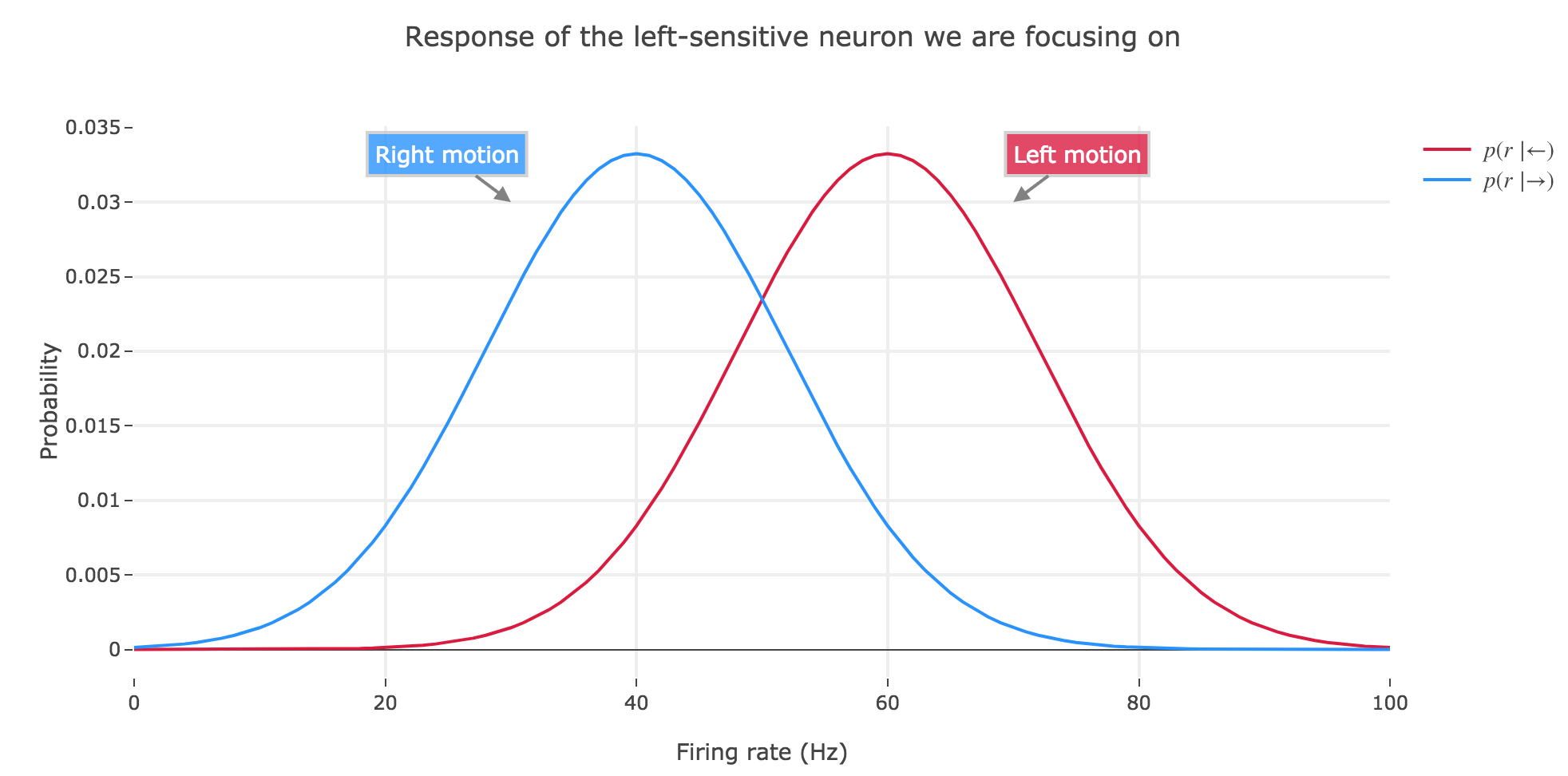
\[p(r) = \frac{1}{\sqrt{2 π σ^2}} \Bigg( p(←) \exp\left(- \frac{(r- μ_←)^2}{2 σ^2}\right) + p(→) \exp\left(- \frac{(r- μ_→)^2}{2 σ^2}\right) \Bigg)\]To use the same example as in the last exercise sheet: if the firing rates range from $0$ to $100$ Hz, and the means and standard deviation are set to be:
- $μ_→ ≝ 60 \textrm{ Hz}$
- $μ_← ≝ 40 \textrm{ Hz}$
- $σ = 12 \textrm{ Hz}$
then we have:
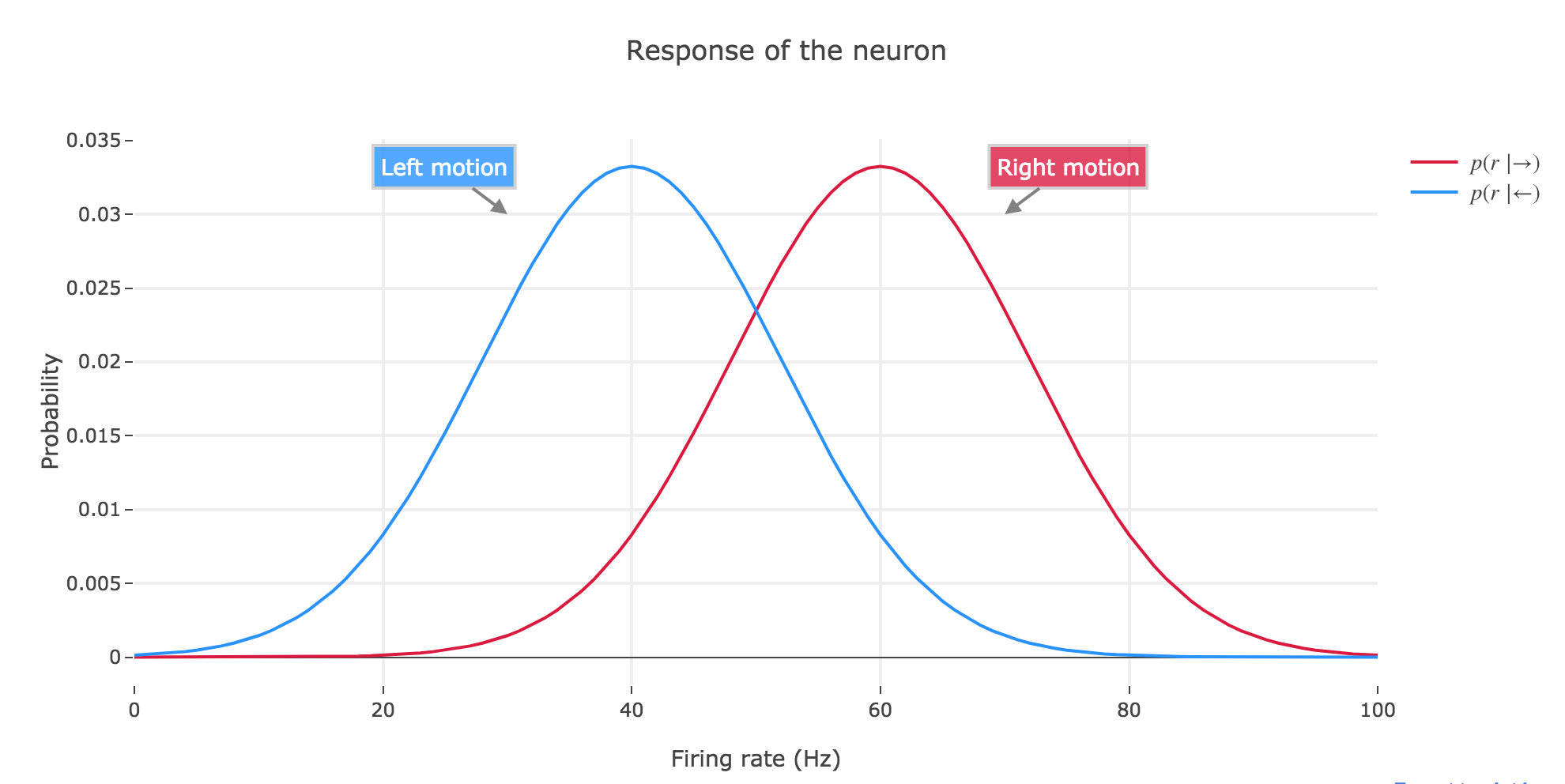
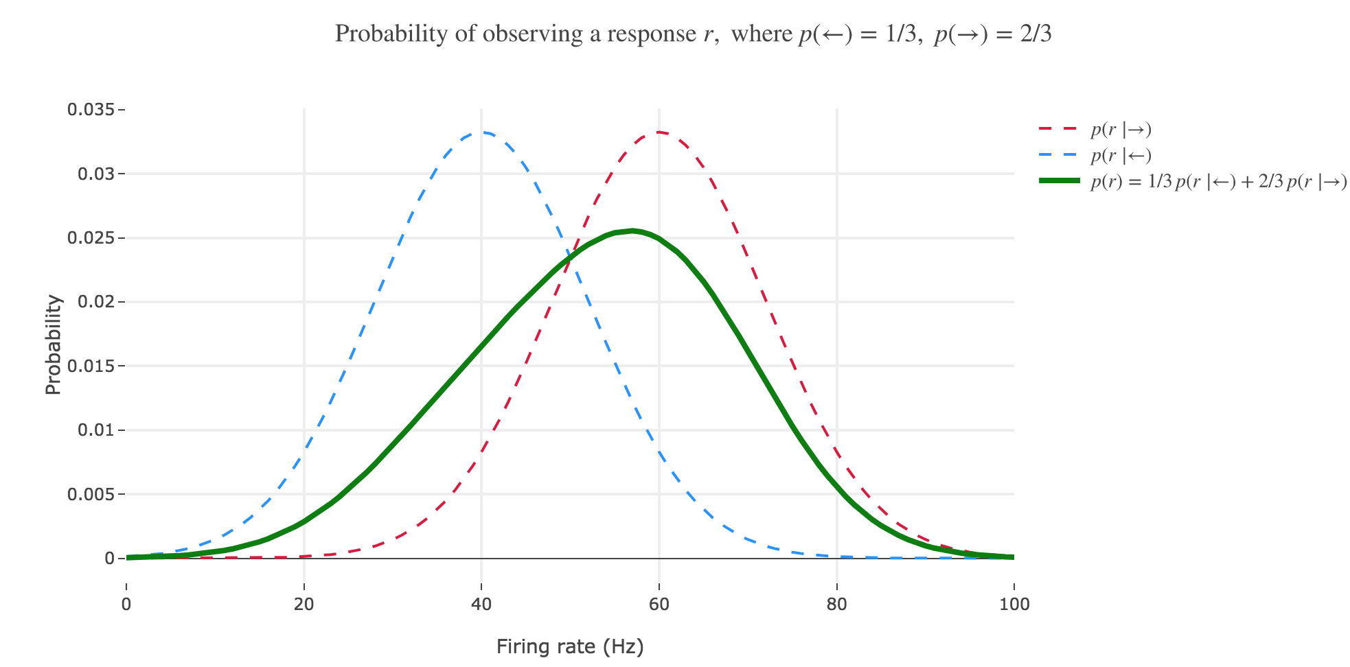
(b) The distribution $p(s \mid r)$ is often called the posterior probability or, for short, the posterior. Calculate the posterior for $s = ←$ and sketch it as a function of $r$, assuming a prior $p(←) = p(→) = 1/2$. Draw the posterior $p(→ \mid r)$ into the same plot.
By Bayes’ theorem:
\[\begin{align*} p(← \mid r) & = \frac{p(r \mid ←)p(←)}{p(r)} \\ & = \frac{p(r \mid ←)p(←)}{p(r \mid ←)p(←) + p(r \mid →)p(→)} \\ & = \frac{1}{1 + \frac{p(r \mid →)p(→)}{p(r \mid ←)p(←)}}\\ & = \frac{1}{1 + \frac{p(r \mid →)}{p(r \mid ←)}}\\ & = \frac{1}{1 + \exp\left(- \frac{(r- μ_→)^2 - (r- μ_←)^2}{2 σ^2}\right)}\\ & = \frac{1}{1 + \exp\left(- \frac{(2r- μ_→ - μ_←)(μ_← - μ_→)}{2 σ^2}\right)}\\ \end{align*}\]So $p(← \mid r)$ is a sigmoid of $\frac{(2r- μ_→ - μ_←)(μ_← - μ_→)}{2 σ^2}$.
As for $p(→ \mid r)$, as $p(\bullet \mid r)$ is a probability distribution:
\[p(→ \mid r) = 1 - p(← \mid r)\]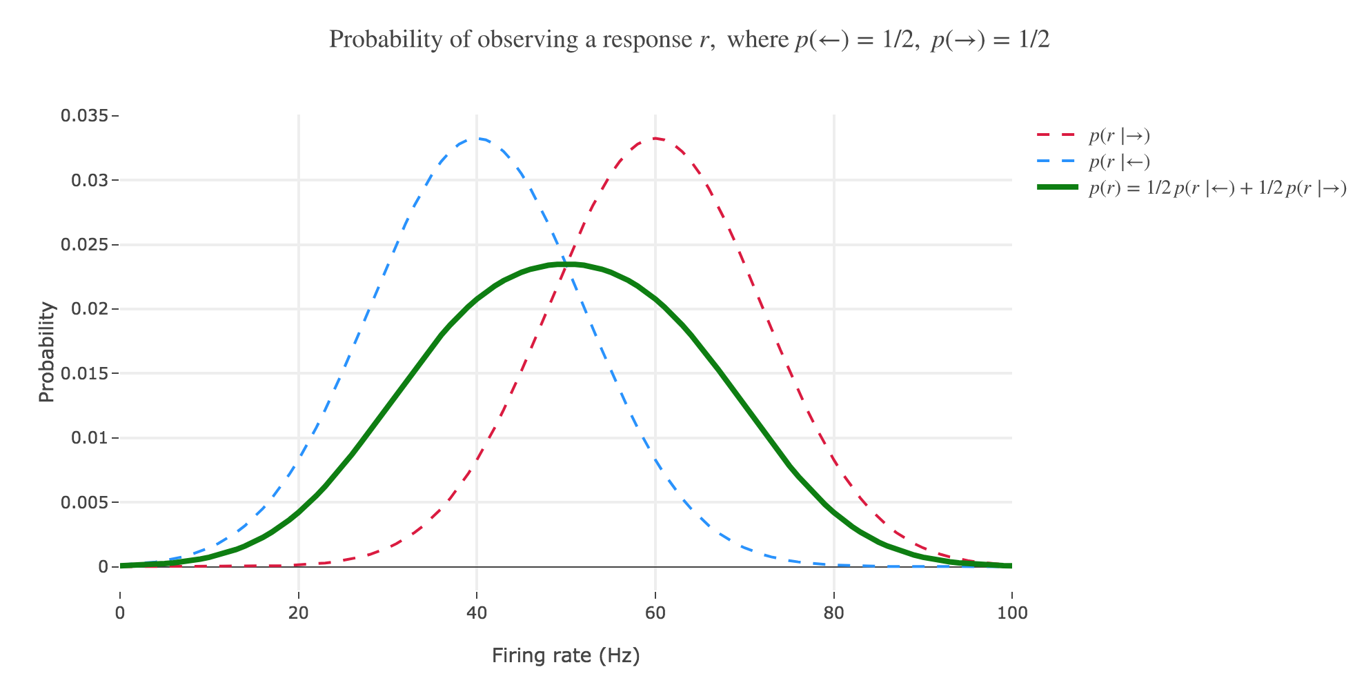
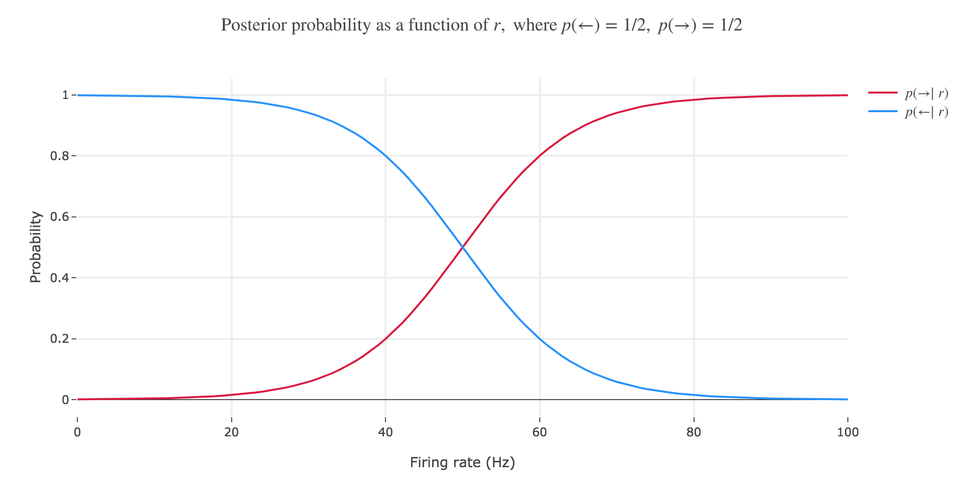
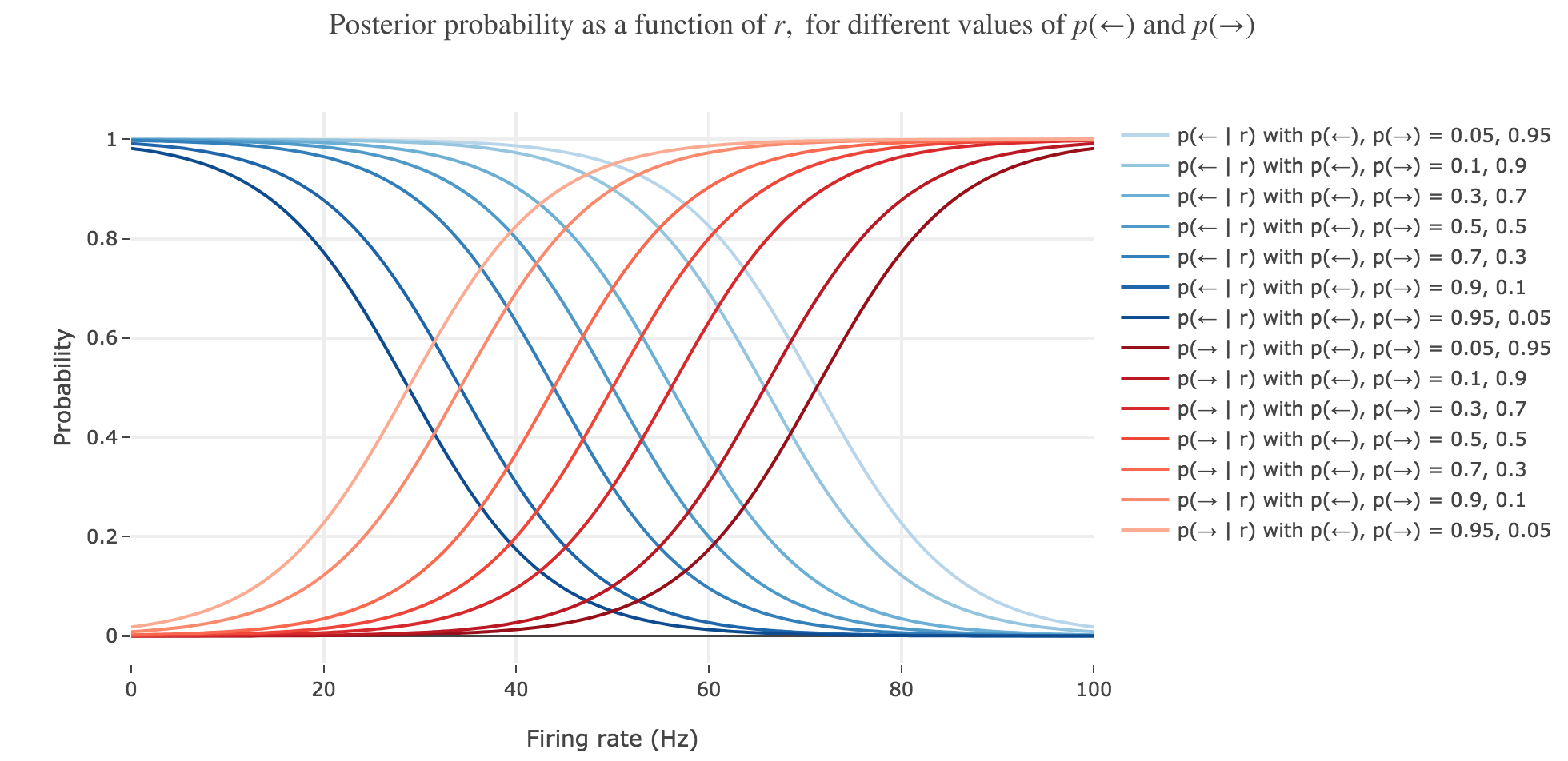
( c) What happens if you change the prior? Investigate how the posterior changes if $p(←)$ becomes much larger than $p(→)$ and vice versa. Make a sketch similar to (b).
If the prior changes, the ratio $\frac{p(→)}{p(←)}$ is no longer equal to $1$ and the posterior changes as well, insofar as the general expression of $p(← \mid r)$ is:
\[\begin{align*} p(← \mid r) & = \frac{1}{1 + \frac{p(→)}{p(←)} \exp\left(- \frac{(2r- μ_→ - μ_←)(μ_← - μ_→)}{2 σ^2}\right)}\\ & = \frac{1}{1 + \exp\left(- \frac{(2r- μ_→ - μ_←)(μ_← - μ_→)}{2 σ^2} + \ln\left(\frac{p(→)}{p(←)}\right) \right)} = 1 - p(→ \mid r) \\ \end{align*}\]As a matter of fact:
-
if $p(←) » p(→)$ (for a fixed $r$):
\[p(← \mid r) ≃ 1 - \frac{p(→)}{p(←)} \exp\left(- \frac{(2r- μ_→ - μ_←)(μ_← - μ_→)}{2 σ^2}\right) \xrightarrow[\frac{p(→)}{p(←)} \to 0^+]{} 1\] -
if $p(←) « p(→)$ (for a fixed $r$):
\[p(← \mid r) \xrightarrow[\frac{p(→)}{p(←)} \to +∞]{} 0^+\]
(d) Let us assume that we decide for leftward motion whenever $r > \frac 1 2 (μ_← + μ_→)$. Interpret this decision rule in the plots above. How well does this rule do depending on the prior? What do you lose when you move from the full posterior to a simple decision (decoding) rule?
NB: the decision rule mentioned in the problem statement suggests that $μ_← > μ_→$, i.e. we are now considering a neuron whose tuning is such that is fires more strongly if the motion stimulus moves leftwards. As nothing was specified before, the example neuron we were focusing on so far was of opposite tuning. We will, from now on, switch to a neuron such that: $μ_← > μ_→$
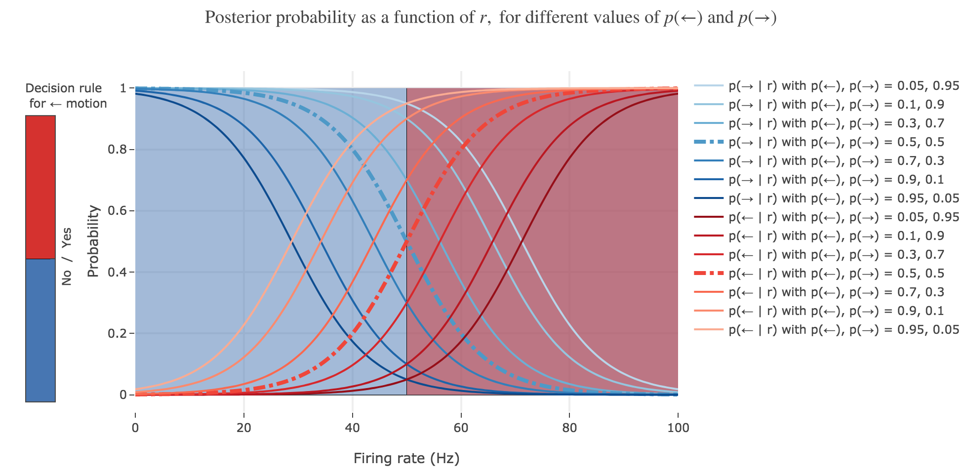
The $r > \frac 1 2 (μ_← + μ_→)$ decision rule corresponds to inferring that the motion is to the left (resp. to the right) in the red (resp. blue) area of figure 2.d.2, which is perfectly suited to the case where $p(←) = p(→) = 1/2$ (bold dash-dotted curves).
However, it does a poor job at predicting the motion direction in the other cases, since it does not take into account the changing prior.
To infer a more sensible rule, let us reconsider the situation: we want to come up with a threshold rate $r_{th}$ such that an ideal observer - making the decision that the motion that caused the neuron to fire at $r > r_{th}$ was to the left (preferred direction of the neuron) - would have a higher chance of being right than wrong. In other words, the decision rule we are looking for is:
\[p(← \mid r) > p(→ \mid r)\]As such, $r_{th}$ satisfies:
\[\begin{align*} & p(← \mid r_{th}) = p(→ \mid r_{th}) \\ ⟺ \; & p(← \mid r_{th}) = 1/2 \\ ⟺ \; & \exp\left(- \frac{(2r_{th}- μ_→ - μ_←)(μ_← - μ_→)}{2 σ^2} + \ln\left(\frac{p(→)}{p(←)}\right)\right) = 1 \\ ⟺ \; & r_{th} = \frac{σ^2}{μ_← - μ_→} \ln\left(\frac{p(→)}{p(←)}\right) + \frac{μ_← + μ_→}{2} \end{align*}\]A more sensible decoding rule would then be:
\[r > \frac{σ^2}{μ_← - μ_→} \ln\left(\frac{p(→)}{p(←)}\right) + \frac{μ_← + μ_→}{2}\]
NB: we can check that, in case $p(→) = p(←)$, we do recover the previous rule.
However, moving from the full posterior to a simple decision rule makes us lose the information relating to how much we are sure about the decision made. Indeed, the full content of the information is contained in the posterior values $p(← \mid r)$ and $p(→ \mid r)$. If $p(← \mid r) > p(→ \mid r)$, then there is a higher chance that the motion that caused the neuron to fire was to the left, but just stating that doesn’t tell you how much higher. You need $p(← \mid r)$ and $p(→ \mid r)$ to do so: as it happens, the chance of leftward motion is $\frac{p(← \mid r)}{p(→ \mid r)}$ times higher.
3. Linear discriminant analysis
Let us redo the calculations for the case of $N$ neurons. If we denote by $\textbf{r}$ the vector of firing rates, Bayes’ theorem reads:
\[p(s \mid \textbf{r})= \frac{p(\textbf{r} \mid s) p(s)}{p(\textbf{r})}\]We assume that the distribution of firing rates again follows a Gaussian so that:
\[p(\textbf{r} \mid s) = \frac{1}{(2π)^{N/2} \sqrt{\det \textbf{C}}} \, \exp\left(- \frac 1 2 (\textbf{r} - \textbf{μ}_s)^T \textbf{C}^{-1} (\textbf{r} - \textbf{μ}_s)\right)\]where
- $\textbf{μ}_s$ denotes the mean of the density for stimulus $s ∈ \lbrace ←, → \rbrace$
- $\textbf{C}$ is the covariance matrix assumed identical for both stimuli
(a) Compute the log-likelihood ratio
\[l(\textbf{r}) ≝ \ln \frac{p(\textbf{r} \mid ←)}{p(\textbf{r} \mid →)}\] \[\begin{align*} l(\textbf{r}) & = \ln\left(\frac{\frac{1}{(2π)^{N/2} \sqrt{\det \textbf{C}}} \, \exp\left(- \frac 1 2 (\textbf{r} - \textbf{μ}_←)^T \textbf{C}^{-1} (\textbf{r} - \textbf{μ}_←)\right)}{\frac{1}{(2π)^{N/2} \sqrt{\det \textbf{C}}} \, \exp\left(- \frac 1 2 (\textbf{r} - \textbf{μ}_→)^T \textbf{C}^{-1} (\textbf{r} - \textbf{μ}_→)\right)}\right) \\ & = \ln\left(\frac{\exp\left(- \frac 1 2 (\textbf{r} - \textbf{μ}_←)^T \textbf{C}^{-1} (\textbf{r} - \textbf{μ}_←)\right)}{\exp\left(- \frac 1 2 (\textbf{r} - \textbf{μ}_→)^T \textbf{C}^{-1} (\textbf{r} - \textbf{μ}_→)\right)}\right) \\ & = \ln\left(\exp\left(- \frac 1 2 (\textbf{r} - \textbf{μ}_←)^T \textbf{C}^{-1} (\textbf{r} - \textbf{μ}_←)\right) \right) - \ln\left(\exp\left(- \frac 1 2 (\textbf{r} - \textbf{μ}_→)^T \textbf{C}^{-1} (\textbf{r} - \textbf{μ}_→)\right)\right) \\ &= \frac 1 2 (\textbf{r} - \textbf{μ}_→)^T \textbf{C}^{-1} (\textbf{r} - \textbf{μ}_→)- \frac 1 2 (\textbf{r} - \textbf{μ}_→)^T \textbf{C}^{-1} (\textbf{r} - \textbf{μ}_→)\\ &= \frac 1 2 \Big(\textbf{r}^T \textbf{C}^{-1} \textbf{r} + \textbf{μ}_→^T \textbf{C}^{-1} \textbf{μ}_→ - \textbf{r}^T \textbf{C}^{-1} \textbf{μ}_→ - \textbf{μ}_→^T \textbf{C}^{-1} \textbf{r} \\ & \quad \; \; - \textbf{r}^T \textbf{C}^{-1} \textbf{r} - \textbf{μ}_←^T \textbf{C}^{-1} \textbf{μ}_← + \textbf{r}^T \textbf{C}^{-1} \textbf{μ}_← + \textbf{μ}_←^T \textbf{C}^{-1} \textbf{r}\Big)\\ & = \frac 1 2 \Big(\textbf{μ}_→^T \textbf{C}^{-1} \textbf{μ}_→ - \textbf{μ}_←^T \textbf{C}^{-1} \textbf{μ}_← - (\textbf{r}^T \textbf{C}^{-1} \textbf{μ}_→ + \textbf{μ}_→^T \textbf{C}^{-1} \textbf{r}) + (\textbf{r}^T \textbf{C}^{-1} \textbf{μ}_← + \textbf{μ}_←^T \textbf{C}^{-1} \textbf{r})\Big)\\ \end{align*}\]But:
- $ℝ \ni \textbf{r}^T \textbf{C}^{-1} \textbf{μ}_s = (\textbf{r}^T \textbf{C}^{-1} \textbf{μ}_s)^T = \textbf{μ}_s^T (\textbf{C}^{-1})^T \textbf{r}$
- since $\textbf{C}$ is a covariance matrix, it is symmetric, hence: $\textbf{C}^T (\textbf{C}^{-1})^T = (\textbf{C}^{-1} \textbf{C})^T = \mathbf{I}^T = \mathbf{I}$, and $(\textbf{C}^{-1})^T = (\textbf{C}^T)^{-1}$
Therefore:
\[\begin{align*} l(\textbf{r}) & = \frac 1 2 \Big(\textbf{μ}_→^T \textbf{C}^{-1} \textbf{μ}_→ - \textbf{μ}_←^T \textbf{C}^{-1} \textbf{μ}_← - 2 \textbf{r}^T \textbf{C}^{-1} \textbf{μ}_→ + 2 \textbf{r}^T \textbf{C}^{-1} \textbf{μ}_← \Big) \end{align*}\]and
\[l(\textbf{r}) = \underbrace{\frac 1 2 \Big(\textbf{μ}_→^T \textbf{C}^{-1} \textbf{μ}_→ - \textbf{μ}_←^T \textbf{C}^{-1} \textbf{μ}_← \Big)}_{≝ \; α_←} + \textbf{r}^T \underbrace{\textbf{C}^{-1} (\textbf{μ}_← - \textbf{μ}_→)}_{≝ \; \textbf{β}_←}\]
(b) Assume that $l(\textbf{r}) = 0$ is the decision boundary, so that any firing rate vector $\textbf{r}$ giving a log-likelihood ratio larger than zero is classified as coming from the stimulus $←$. Compute a formula for the decision boundary. What shape does this boundary have?
First, let us show how we could come up with the $l(\textbf{r}) > 0$ decision boundary.
\[\begin{align*} & p(← \mid \textbf{r}) > p(→ \mid \textbf{r}) \\ ⟺ \; & \frac{p(← \mid \textbf{r})}{p(→ \mid \textbf{r})} > 1 \\ ⟺ \; & \frac{p(\textbf{r} \mid ←) p(←)/p(\textbf{r})}{p(\textbf{r} \mid →) p(→)/p(\textbf{r})} > 1 \\ ⟺ \; & \frac{p(\textbf{r} \mid ←)}{p(\textbf{r} \mid →)} > \frac{p(→)}{p(←)} \\ ⟺ \; & \frac{p(\textbf{r} \mid ←)}{p(\textbf{r} \mid →)} > \frac{p(→)}{p(←)} \\ ⟺ \; & l(\textbf{r}) ≝ \ln \left(\frac{p(\textbf{r} \mid ←)}{p(\textbf{r} \mid →)}\right) > \ln\left(\frac{p(→)}{p(←)}\right) \\ \end{align*}\]So the $l(\textbf{r}) > 0$ decision boundary is a good one if and only if \(\ln\left(\frac{p(→)}{p(←)}\right) = 0 ⟺ p(→) = p(←) = 1/2\)
The formula for this decision boundary is the following one:
\(l(\textbf{r}) = 0 ⟺ \underbrace{\frac 1 2 \Big(\textbf{μ}_→^T \textbf{C}^{-1} \textbf{μ}_→ - \textbf{μ}_←^T \textbf{C}^{-1} \textbf{μ}_← \Big)}_{≝ \; α_←} + \textbf{r}^T \underbrace{\textbf{C}^{-1} (\textbf{μ}_← - \textbf{μ}_→)}_{≝ \; \textbf{β}_←} = 0 \\ ⟺ \textbf{r}^T \textbf{β}_← = - α_←\) It’s an affine hyperplane (i.e. a subspace of codimension $1$) in the $n$-dimensional space $ℝ^n$.
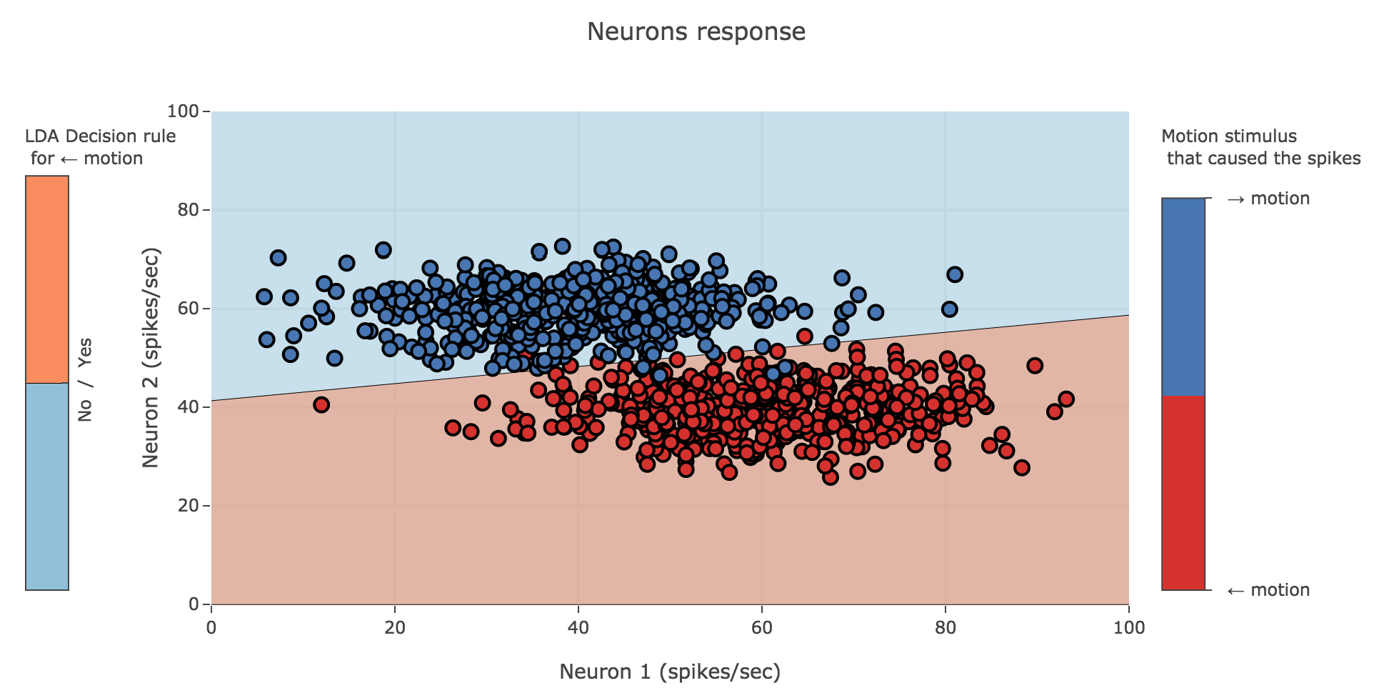
( c) Assume that $p(←) = p(→) = 1/2$. Assume we are analyzing two neurons with uncorrelated activities, so that the covariance matrix is:
\[\textbf{C} = \begin{pmatrix} σ_1^2 & 0 \\ 0 & σ_2^2 \\ \end{pmatrix}\]Sketch the decision boundary for this case.
With:
- $\textbf{μ}_← ≝ (60 \text{ Hz}, 40 \text{ Hz})$
- $\textbf{μ}_→ ≝ (40 \text{ Hz}, 60 \text{ Hz})$
- $\textbf{C} ≝ \begin{pmatrix}
12^2 \text{ Hz}^2 & 0
0 & 5^2 \text{ Hz}^2
\end{pmatrix}$
we get, by resorting to the LDA decision boundary $l(\textbf{r}) = \textbf{r}^T \textbf{β}← + α← > 0$:
Leave a comment