Exercise Sheet 3: Signal Detection Theory & Reinforcement Learning
Exercise Sheet 3: Signal Detection Theory & Reinforcement Learning
Younesse Kaddar
1. Signal Detection Theory
Consider the two-alternative-choice motion discrimination task in which the subject has to determine the direction of motion of a stimulus. As ideal observers, we obtain access to two neurons with opposite tuning (so that e.g. neuron 1 will fire more strongly than neuron 2 if the motion stimulus moves leftwards, and neuron 2 more strongly than neuron 1 if the motion stimulus moves rightwards).
If the motion was
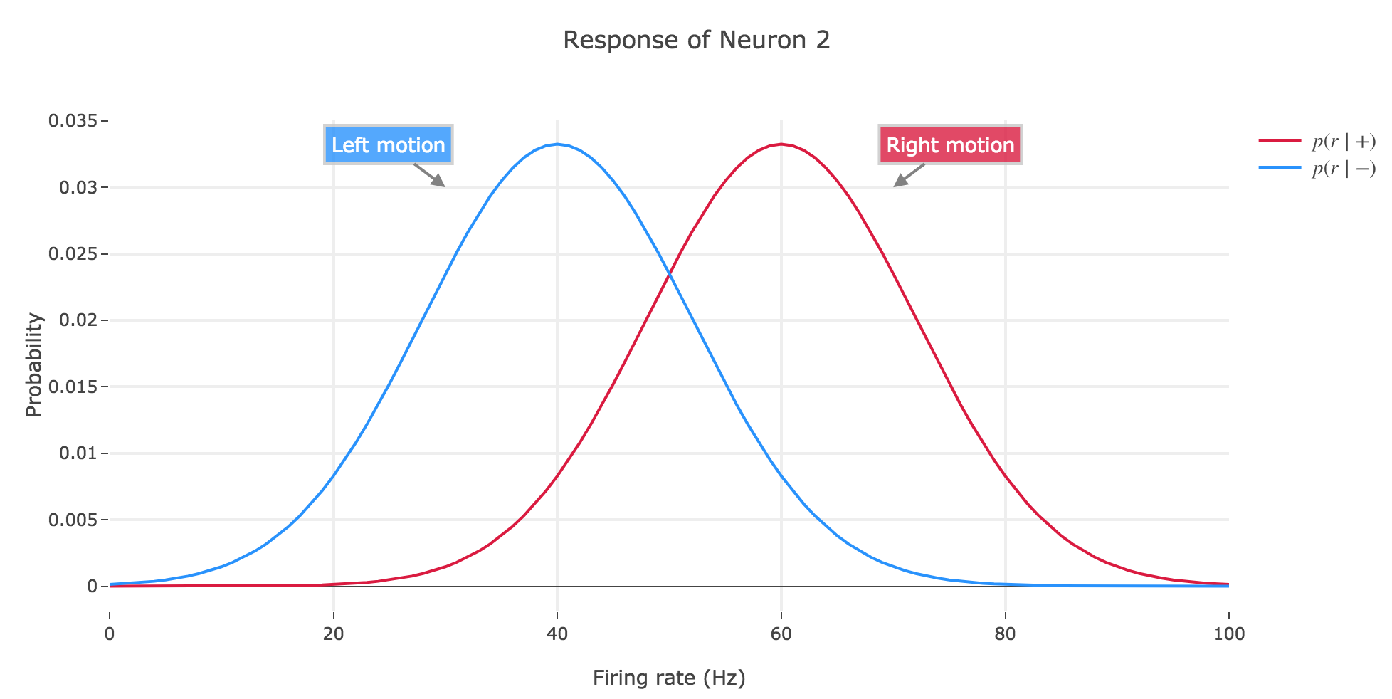
- to the left ($+$): then the firing rates of neuron 1 follow the distribution $p(r \mid +)$ and those of neuron 2 the distribution $p(r \mid -)$
- to the right ($-$): then neuron 1 fires according to $p(r \mid -)$ and neuron 2 according to $p(r \mid +)$
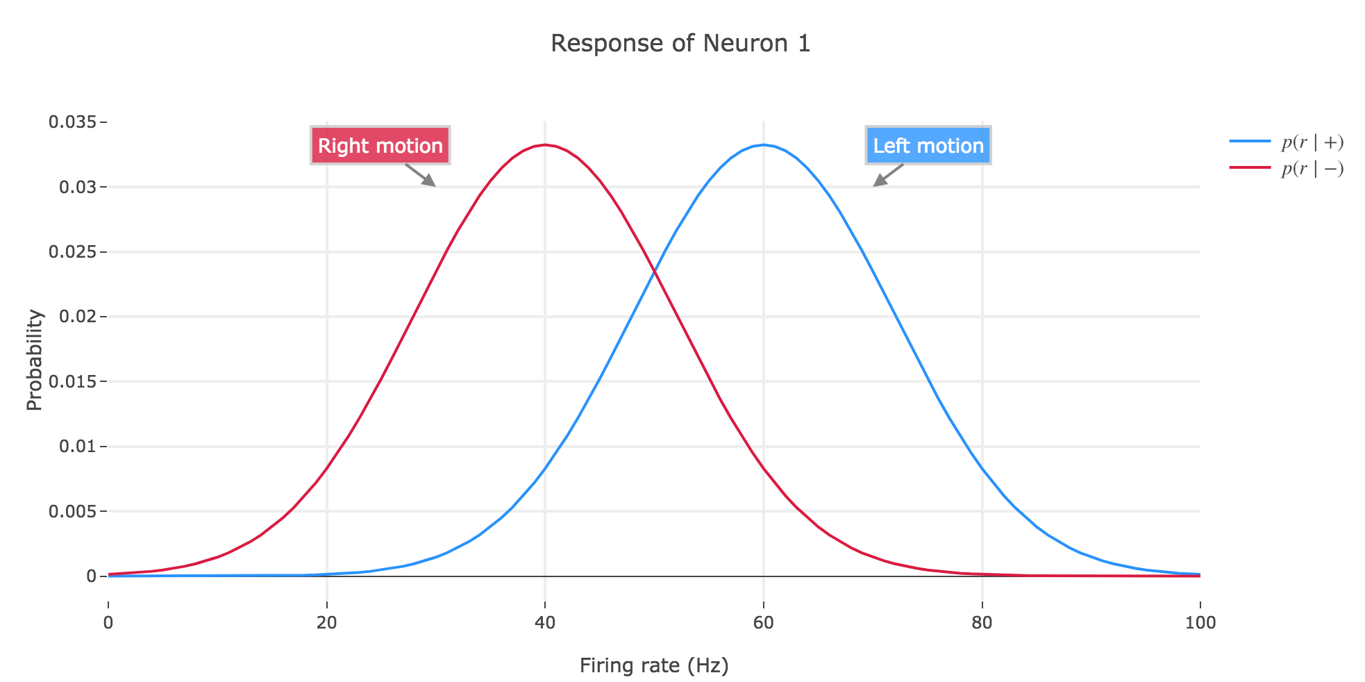
a) Assume that the distribution $p(r \mid +)$ and $p(r \mid -)$ are Gaussian and sketch the above scenario (two neurons, two possible stimuli)
For instance, if the firing rates range from $0$ to $100$ Hz, and if the mean and standard deviation $μ_+, σ_+$ (resp. $μ_-, σ_-$) of $p(r \mid +)$ (resp. $p(r \mid -)$) are set to be:
- $μ_+ ≝ 60, σ_+ = 12$
- $μ_- ≝ 40, σ_- = 12$
to resemble the example seen in class, then we have:
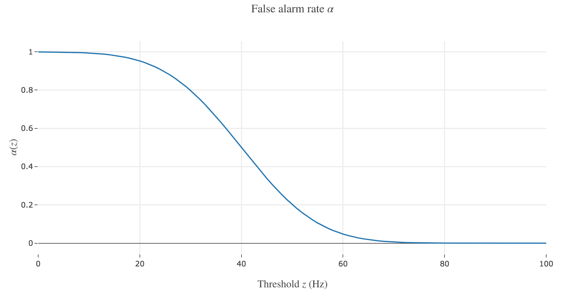
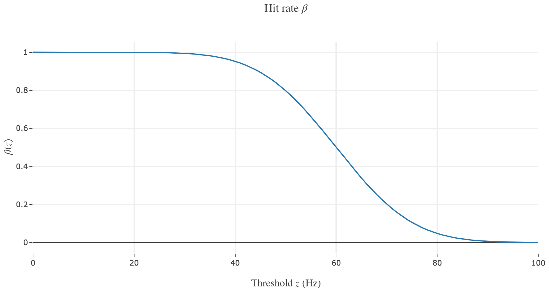
b) In class, we introduced the two functions
\[\begin{cases} α(z) ≝ p(r ≥ z \mid -)\\ β(z) ≝ p(r ≥ z \mid +) \end{cases}\]Sketch these functions. What do they indicate in the present context?
Let us call preferred direction of a neuron the left (resp. right) one for neuron 1 (resp. for neuron 2): that is, the direction that causes the neuron to fire more strongly than the other.
The probability $α(z) ≝ p(r ≥ z \mid -) = \int_z^{+∞} p(\bullet \mid -)$ for the decision threshold $z$ is a false alarm rate, i.e. the probability that an ideal observer, observing neuron $i ∈ \lbrace 1, 2 \rbrace$, would mistakenly make the decision that the motion that caused neuron $i$ to fire above the threshold $z$ was to the preferred direction of neuron $i$, while in fact it was in the other direction.
The probability $β(z) ≝ p(r ≥ z \mid +) = \int_z^{+∞} p(\bullet \mid +)$ for the decision threshold $z$ is a hit rate, i.e. the probability that an ideal observer, observing neuron $i ∈ \lbrace 1, 2 \rbrace$, would rightly make the decision that the motion that caused neuron $i$ to fire above the threshold $z$ was to the preferred direction of neuron $i$, while it was indeed in this direction.
c) Compute the derivatives $\frac{ {\rm d} α}{ {\rm d}z}(z)$ and $\frac{ {\rm d} β}{ {\rm d} z}(z)$.
\[\begin{align*} \frac{ {\rm d} α}{ {\rm d}z}(z) & = \frac{ {\rm d}}{ {\rm d}z} \left(\int_z^{+∞} p(\bullet \mid -) \right)\\ & = \frac{ {\rm d}}{ {\rm d}z} \left( \Big[P(\bullet \mid -)\Big]_z^{+∞}\right) &&\text{where } P(\bullet \mid -)\text{ is a primitive of } p(\bullet \mid -) \\ & = \frac{ {\rm d}}{ {\rm d}z} \left( \text{const} - P(z \mid -)\right) \\ & = - \frac{ {\rm d}}{ {\rm d}z} P(z \mid -)\\ & = - p(z \mid -) \end{align*}\]And likewise:
\[\frac{ {\rm d} β}{ {\rm d}z}(z) = -p(z \mid +)\]d) Let us call $r_i$ the firing rate of neuron $i ∈ \lbrace 1, 2 \rbrace$. What is the probability $p(r_1, r_2 \mid +)$?
Strictly speaking, there is no such thing as a preferred direction for the pair $\lbrace r_1, r_2 \rbrace$, so there may be a problem of definition when it comes to $p(r_1, r_2 \mid +)$. Based on the introductory part of the problem statement, let us assume that the preferred direction for $\lbrace r_1, r_2 \rbrace$ is the left one.
In this case:
\[\begin{align*} p(r_1, r_2 \mid +) & ≝ p(r_1, r_2 \mid \text{left motion}) \\ & = p(r_1 \mid \text{left motion}) \cdot p(r_2 \mid \text{left motion}) &&⊛\\ & = p(r_1 \mid +) \cdot p(r_2 \mid -) \end{align*}\]The $⊛$ part is due to the events being assumed to be conditionally independent given any fixed stimulus, as seen in class.
Similarly: if the preferred direction of the pair $\lbrace r_1, r_2 \rbrace$ is assumed to be the right one, then:
\[p(r_1, r_2 \mid +) = p(r_1 \mid -) \cdot p(r_2 \mid +)\]e) Advanced: Let’s assume an ideal observer makes the decision “motion was leftwards” whenever $r_1 > r_2$. How often will this observer be correct, assuming that leftwards and rightwards motion occur equally often? Show that the result corresponds to the area under the ROC-curve.
From now on, in compliance with the problem statement, let us assume that the preferred direction for $\lbrace r_1, r_2 \rbrace$ is the left one.
We are asked to compute $p(r_1 > r_2 \mid +)$, that is:
\[\begin{align*} p(r_1 > r_2 \mid +) & = \int\limits_{\lbrace r_1, r_2 \mid r_1 > r_2 \rbrace} p(r_1, r_2 \mid +) {\rm d}r_1 {\rm d}r_2\\ & = \int\limits_0^{+∞} \Bigg( \int\limits_{r_2}^{+∞} \underbrace{p(r_1, r_2 \mid +)}_{= \, p(r_1 \mid +) \cdot p(r_2 \mid -) \;\text{ by d)}} {\rm d}r_1\Bigg) {\rm d}r_2\\ & = \int\limits_0^{+∞} \Bigg( \int\limits_{r_2}^{+∞} \underbrace{p(r_2 \mid -)}_{\rlap{\text{doesn't depend on } r_1}} \; p(r_1 \mid +) {\rm d}r_1\Bigg) {\rm d}r_2\\ & = \int\limits_0^{+∞} p(r_2 \mid -)\, \underbrace{\Bigg( \int\limits_{r_2}^{+∞} \; p(r_1 \mid +) {\rm d}r_1\Bigg)}_{≝ \, β(r_2)} {\rm d}r_2\\ & = \int\limits_0^{+∞} β(r_2) \; \underbrace{p(r_2 \mid -)}_{= \, - α'(r_2) \;\text{ by c)}} {\rm d}r_2\\ & = \int\limits_{+∞}^0 β(r_2) \; α'(r_2) {\rm d}r_2\\ \end{align*}\]And as
\[\begin{cases} \lim\limits_{r_2 → +∞} α(r_2) = 0 \\ α(0) = 1 \end{cases}\]we conclude, by u-substitution, that:
\[p(r_1 > r_2 \mid +) = \int_0^1 β(α) {\rm d}α \, ≝ \text{AUC}\]which is the area under the Receiver Operating Characteristic curve.
2. Reinforcement Learning Theory
In the lecture, we learned that the reinforcement learning framework allows an agent to learn the optimal sequence of choices in a given envrionment (optimal in the sense that the agent will gather the maximum amount of reward).
This framework is very powerful and could in principle learn many things (e.g. playing chess), even if this may often be impractical.
What are environmental scenarios which this framework, as presented in the lecture, will never be able to learn? If you can think of a scenario, try to illustrate it with a simple example.
Reinforcement Learning (RL) is a simplistic - yet effective - framework which has its fair share of limitations. Let us examine some of them.
Curse of dimensionality
One of the most obvious limitation is the curse of dimensionality, as we saw in class, which forces us to go from model-free learning to model-based one. The problem is that there’s no systematic or easy way to come up with a good model that will appropriately generalize: recall the chess linear model example mentioned in the course slides (slide 50), which can actually learn to play chess, but is very bad at doing so. The situation is even worse for the real world examples we deal with in neuroscience, which are far more complex and involve far more parameters than a board game, if we were to model them faithfully.
Markovian/Memorylessness property
Another drawback of the RL framework is the Markovian/memorylessness assumption it is based upon: the next state depends only on the current state and taken action, which is a serious limitation. Indeed, there are countless examples where this assumption does not hold, especially whenever the next state may depend on all the previous taken actions/visited states.
To come back to the “rat in maze” example we saw in class: let us assume the maze has paths of different lengths. The rat may want to return back to its mischief afterwards, and thus may take into account the length of the path taken so far (not to venture too deep into the maze), in which case the next state would depend on all the previously visited states.
Discrete states/actions
Another limitation is that we resort to a discrete set of state and actions. With continuous states and action, in the maze example:
- states may not just be intersections in the maze (discrete), but any point (to look for food at this spot) in a pathway (continuous)
- an action the rat may take may be for example “going in this or that direction for $x ∈ℝ_+$ meters”
Reward function
The reward function (on which the state value function is based) is the cornerstone of the RL framework. However, in practice, how to quantify and even define the reward may not be all that clear. In the maze example, the reward may be thought of as the amount of food found at this or that spot, but the rat may also take into account the attractiveness of spots as potential shelters: in which case: how to faithfully define/quantify the reward?
One single agent in a static envrionment
Finally, it can be stressed that in our RL framework: the agent
- doesn’t interact with other agents
- “has the upper hand” with respect to its envrionment, as it is the one to take action in the environment, which can then be described as static (in real world examples: the environment may be “protean” and change according to parameters that don’t depend only on the agent’s actions)
In our maze example again: the rat may encounter other rats (which may then cause fights, collaboration, etc…), and if the maze is thought of as the sewers for instance: certain spots may become more or less dangerous/unappealing according to different varying factors (luminosity, level of water, etc…).
Leave a comment