[Problem Set 3 Spike trains] Problem 1: Poisson spike trains
Link of the iPython notebook for the code
AT2 – Neuromodeling: Problem set #3 SPIKE TRAINS
PROBLEM 1: Poisson spike trains
Brain neuron emit spikes seemingly randomly: we will aim to model such spike trains, by relying on the following assumptions:
- spike events occur independently of one another
- they occur at a constant firing rate $r$
- there exists a time bin $Δt$ within which no two spikes can be fired
-
within each time span $Δt$, the probability of the neuron firing is $rΔt$.
-
In other words: the random variable $X_t$ whose outcome is $1$ (resp. $0$) if there is a (resp. no) spike between $t$ and $t+Δt$ follows a Bernoulli distribution:
\[X_t \sim ℬ(r Δt)\]
-
1. Generating spike trains
Let $M ≝ T/Δt$, where $T$ is the length (in seconds) of the spike trains we will consider from now on.
In compliance with what we assumed before, a spike train can be modeled as a $M$-dimensional random vector whose $i$-th coordinate (for $0 ≤ i ≤ M-1$) is the output of $X_{i Δt}$ (the values of which are in $\lbrace 0, 1 \rbrace$). In concrete terms, when implementing such a vector of $\lbrace 0, 1 \rbrace^M$: at each coordinate, it has a constant probability to be equal to $1$ ($0$ otherwise).
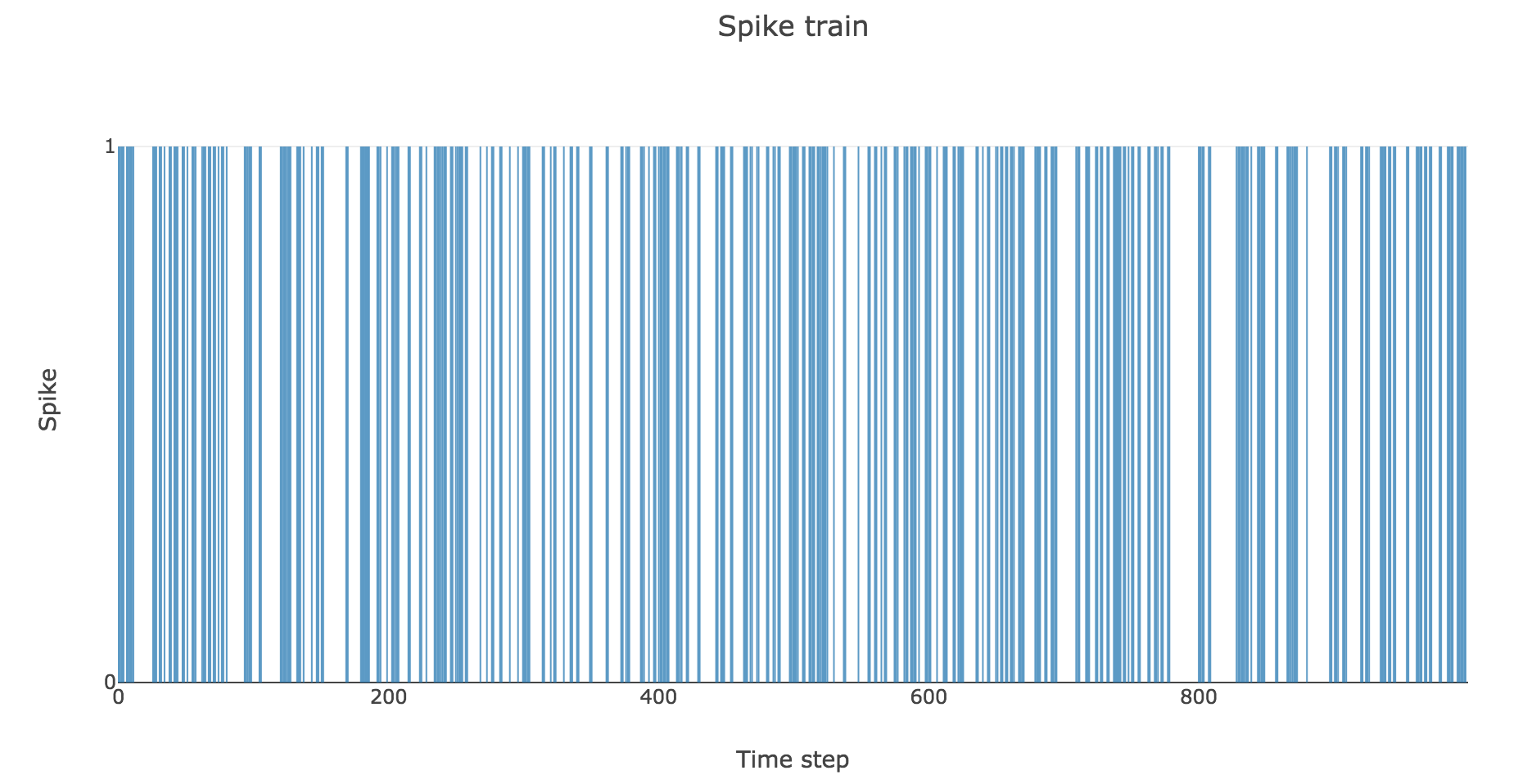
Example: For instance, if on average every fourth element in the vector is made to indicate a spike (i.e. is equal to $1$), that is: the previously mentioned constant probability is equal to $1/4$:
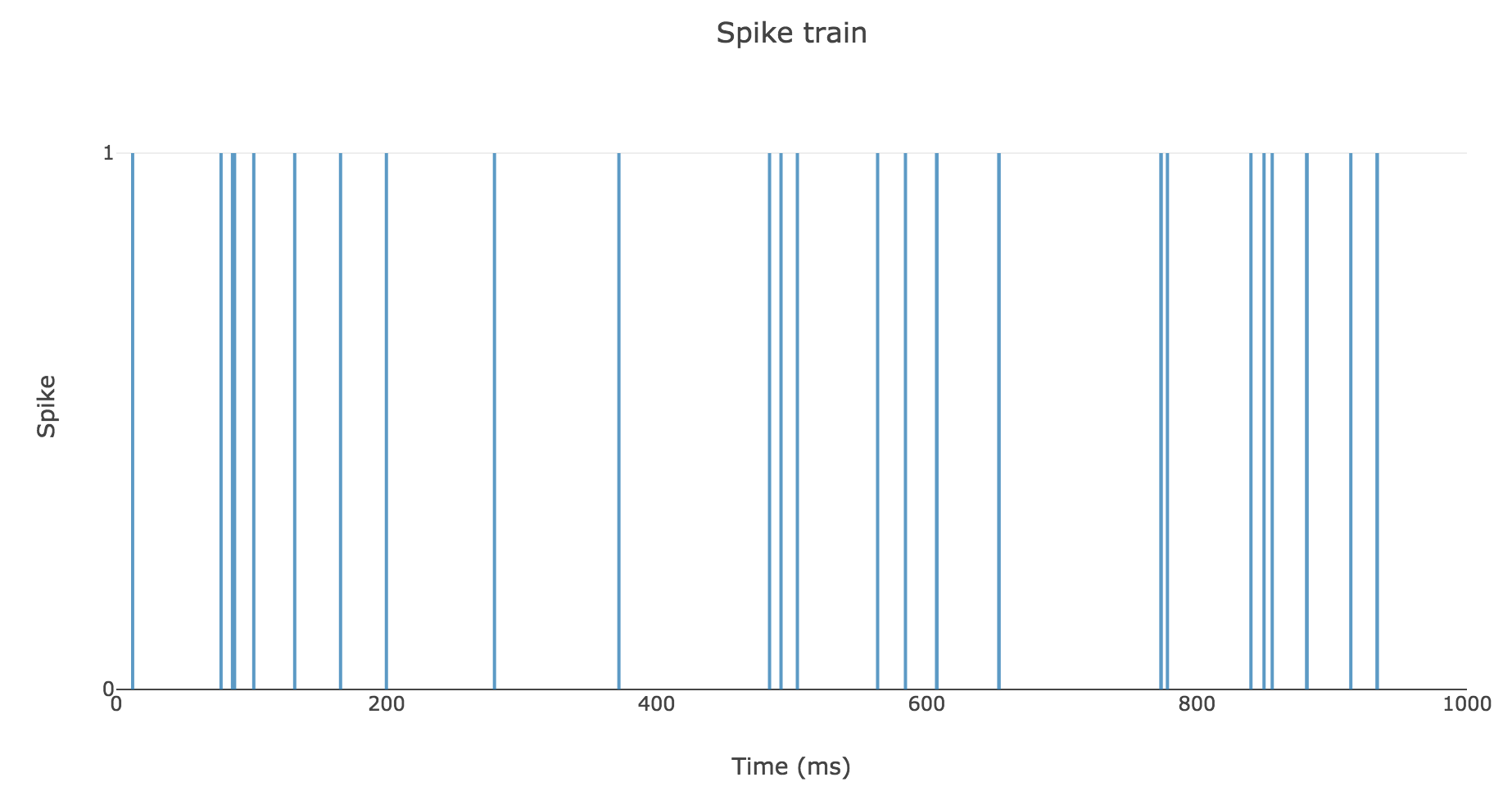
To clarify the time units, let us set
- $Δt ≝ 2 \text{ ms}$
- $T = 1 \text{ s}$
- $r = 25 \text{ spikes/sec}$
Then here is an example of a spike train:
2. Spike counts & Interspike intervals
Now, informative features can be extracted from each spike train, such as:
- its total number of spikes (which gives a global information about the spike train, but have us overlook the time step at which each spike occurred)
- the interspike intervals (which give us local clues on the contrary, but encompass the time-related information we lost with the spike counts only)
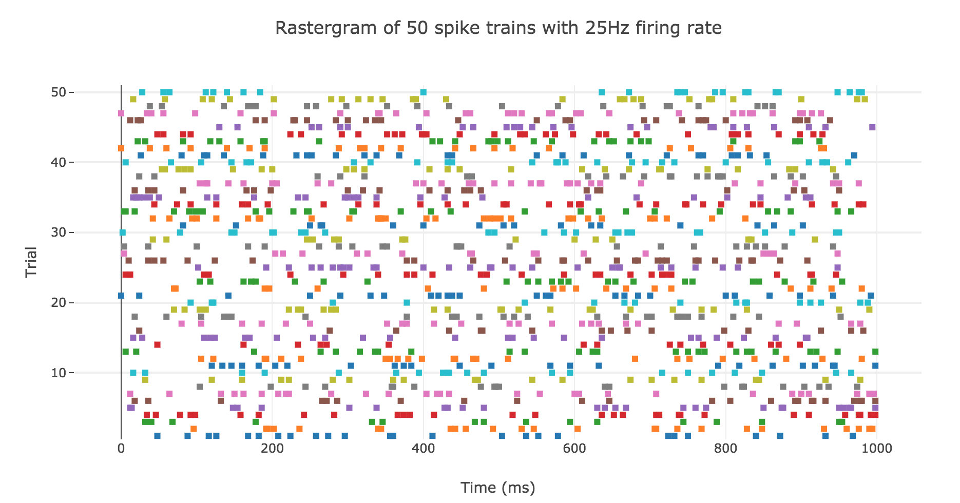
A natural question to ask ourselves is: what is their distribution? To this end, let us generate $N ≝ 200$ spike trains with firing rate $r ≝ 25 \text{ Hz}$.
Here is the rastergram of $50$ of them:
Spike counts
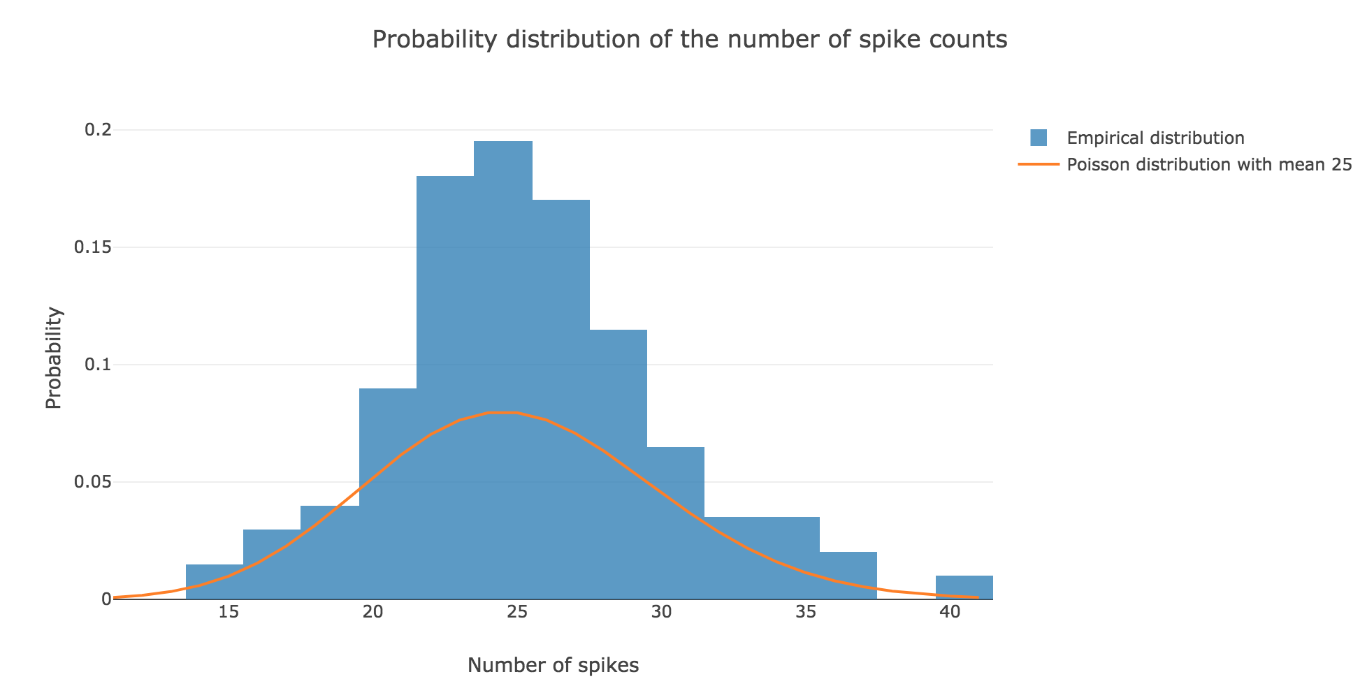
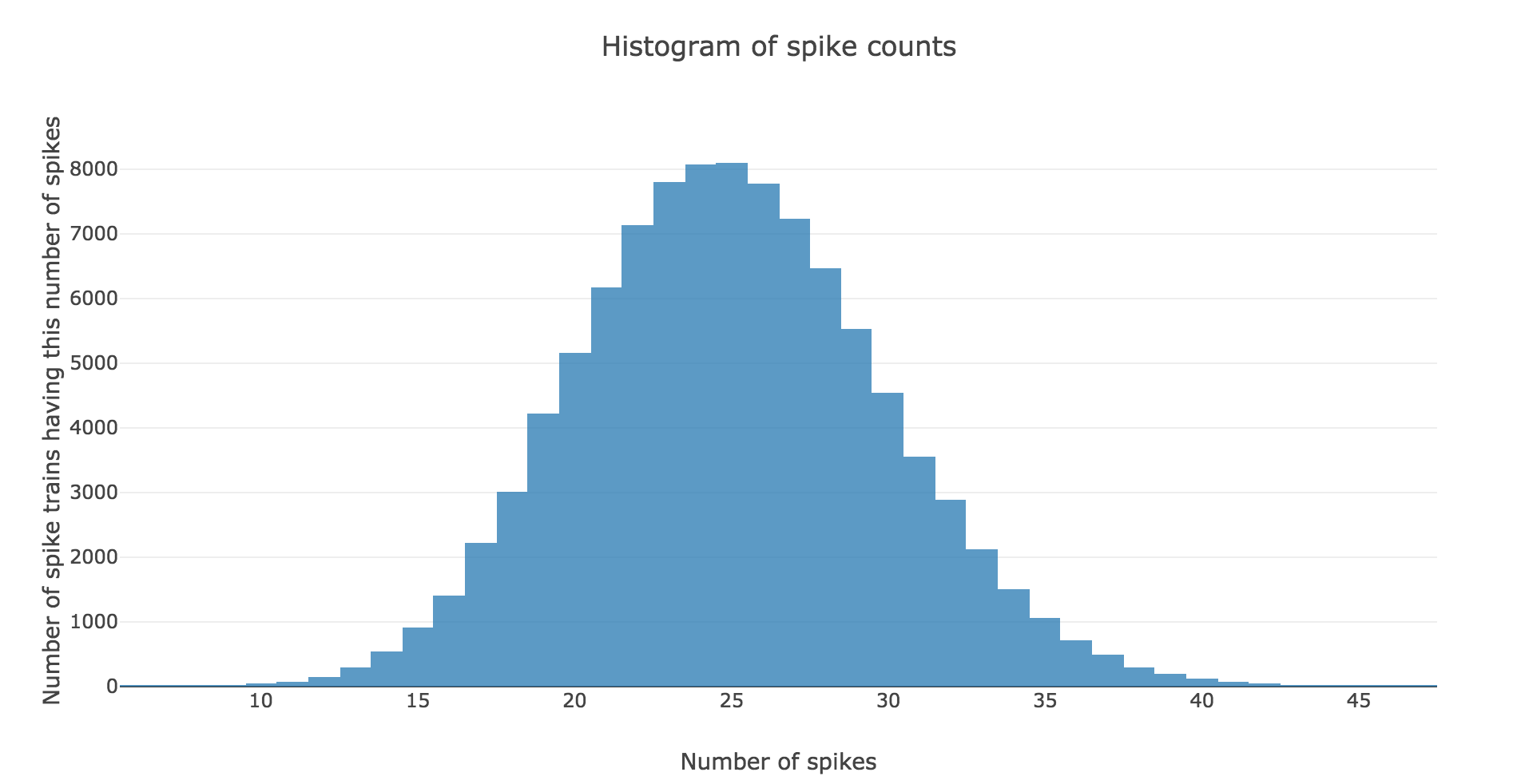
Here is the spike count histogram of all of these $200$ spike trains:
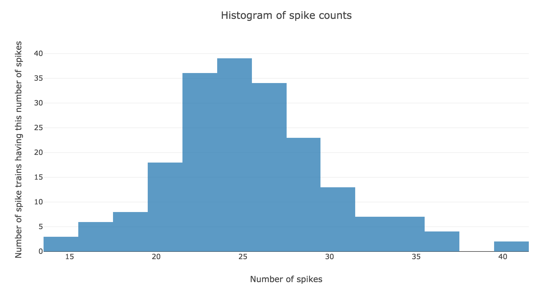
We claim that spike counts are following a Poisson distribution of mean $rT ≝ 25$ (spikes), which may not seem obvious at first sight with so few spike trains:
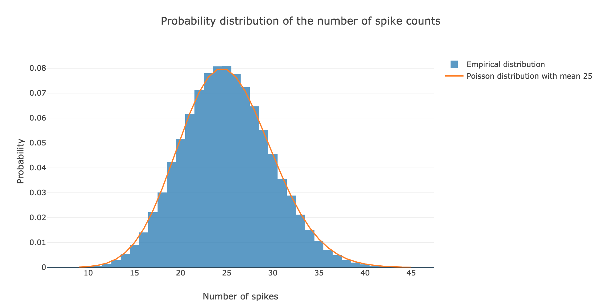
However, it becomes more apparent when the number $N$ of spike trains is increased. For $N ≝ 100000$ for instance:
the spike counts distribution matches very well the Poisson one:
This can be explained theoretically: the assumptions stated in the introduction make the Poisson distribution perfectly suited to model the spike counts distribution. More precisely: by definition, the random variable $X$ counting the number of spikes is binomial:
\[X ≝ \sum\limits_{ n=0 }^{M-1} \underbrace{X_{nΔt}}_{\; \sim \; ℬ(rΔt)} \; \sim \; ℬ(M, rΔt)\]as the $X_t$ are independent (by hypothesis) and identically distributed ($∀t, X_t \sim \; ℬ(rΔt)$).
But it is well known that the Poisson distribution $𝒫(\underbrace{M × rΔt}_{= \, rT})$ successfully approximates such a binomial distribution provided that $M$ is large enough and $rΔt$ is small enough. Here:
- $M ≝ T/Δt = \frac{1000}{2} = 500$
- $rΔt = 25 × 2 \cdot 10^{-3} = 0.05$
which makes the Poisson distribution $𝒫(rT)$, i.e. $𝒫(25)$, perfectly suited to approximate the binomial distribution $ℬ(M, rΔt)$!
Interspike intervals
Here is the interspike interval histogram of $200$ spike trains with firing rate $r ≝ 25 \text{ Hz}$:
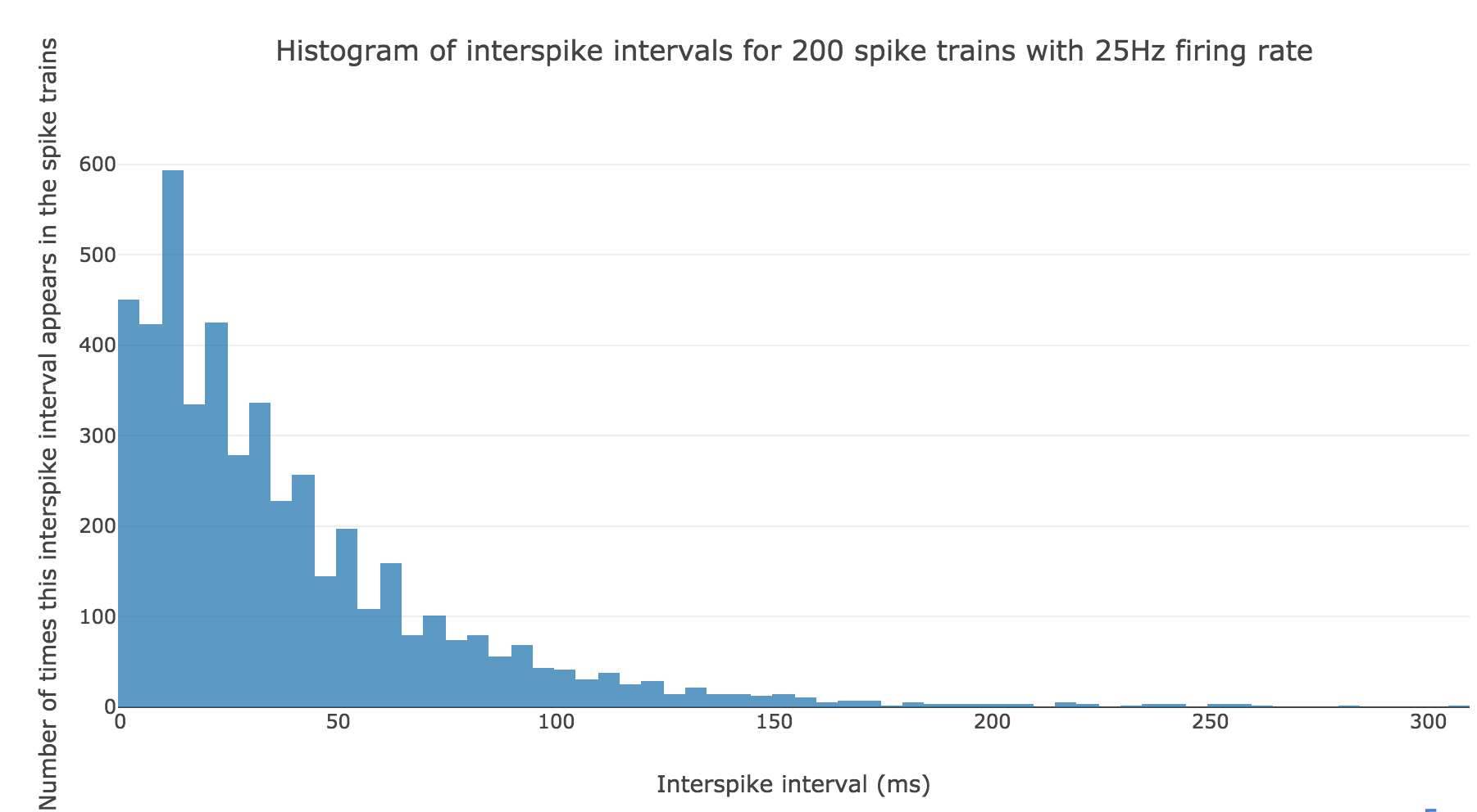
From a theoretical standpoint: if we denote by $Y$ the random variable whose outcome is the length of an interspike interval, in compliance with the assumptions in the introduction, it comes that:
\[\begin{cases} ∀t ≤ 0, \quad P(Y > t) = 1 \\ ∀t > 0, \quad P(Y > t) = (1 - rΔt)^{t/Δt} = \exp\left(\frac{t}{Δt} \ln(1 - rΔt)\right) = \exp\left(- t \, \frac{\ln\left(\frac{1}{1 - rΔt}\right)}{Δt}\right) \end{cases}\]So:
\[\begin{cases} ∀t ≤ 0, \quad P(Y ≤ t) = 0 \\ ∀t > 0, \quad P(Y ≤ t) = 1 - \exp\left(- t \, \ln\left(\frac{1}{1 - rΔt}\right)/Δt\right) \end{cases}\]Therefore, by definition of its cumulative distribution function, the interspike interval variable $Y$ follows an exponential distribution of rate $\ln\left(\frac{1}{1 - rΔt}\right)/Δt$
Leave a comment