Problem Set 3: Spike trains

AT2 – Neuromodeling: Problem set #3 SPIKE TRAINS

Younesse Kaddar

PROBLEM 1: Poisson spike trains

Link of the iPython notebook for the code

Brain neuron emit spikes seemingly randomly: we will aim to model such spike trains, by relying on the following assumptions:

1. spike events occur independently of one another
2. they occur at a constant firing rate $r$
3. there exists a time bin $Δt$ within which no two spikes can be fired

4. within each time span $Δt$, the probability of the neuron firing is $rΔt$.

   • In other words: the random variable $X_t$ whose outcome is $1$ (resp. $0$) if there is a (resp. no) spike between $t$ and $t+Δt$ follows a Bernoulli distribution:

     \[X_t \sim ℬ(r Δt)\]

1. Generating spike trains

Let $M ≝ T/Δt$, where $T$ is the length (in seconds) of the spike trains we will consider from now on.

In compliance with what we assumed before, a spike train can be modeled as a $M$-dimensional random vector whose $i$-th coordinate (for $0 ≤ i ≤ M-1$) is the output of $X_{i Δt}$ (the values of which are in $\lbrace 0, 1 \rbrace$). In concrete terms, when implementing such a vector of $\lbrace 0, 1 \rbrace^M$: at each coordinate, it has a constant probability to be equal to $1$ ($0$ otherwise).

Example: For instance, if on average every fourth element in the vector is made to indicate a spike (i.e. is equal to $1$), that is: the previously mentioned constant probability is equal to $1/4$:

Figure a. - Spike train such that there is a spike every fourth time bin on average

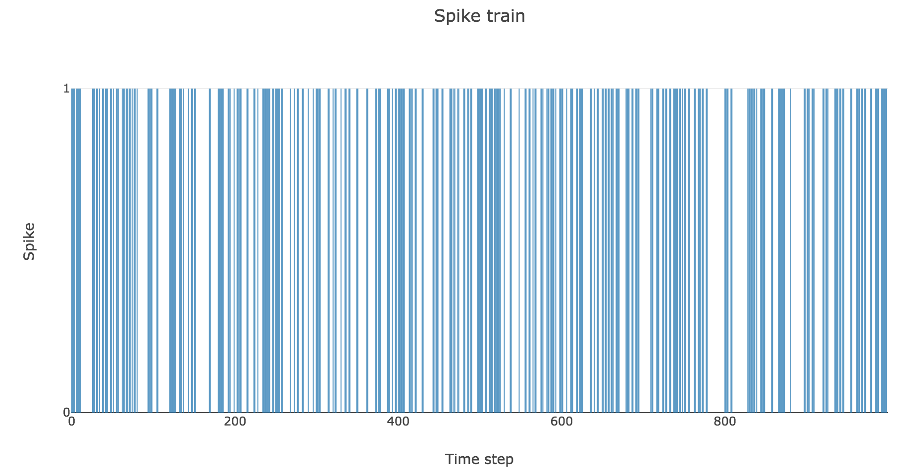
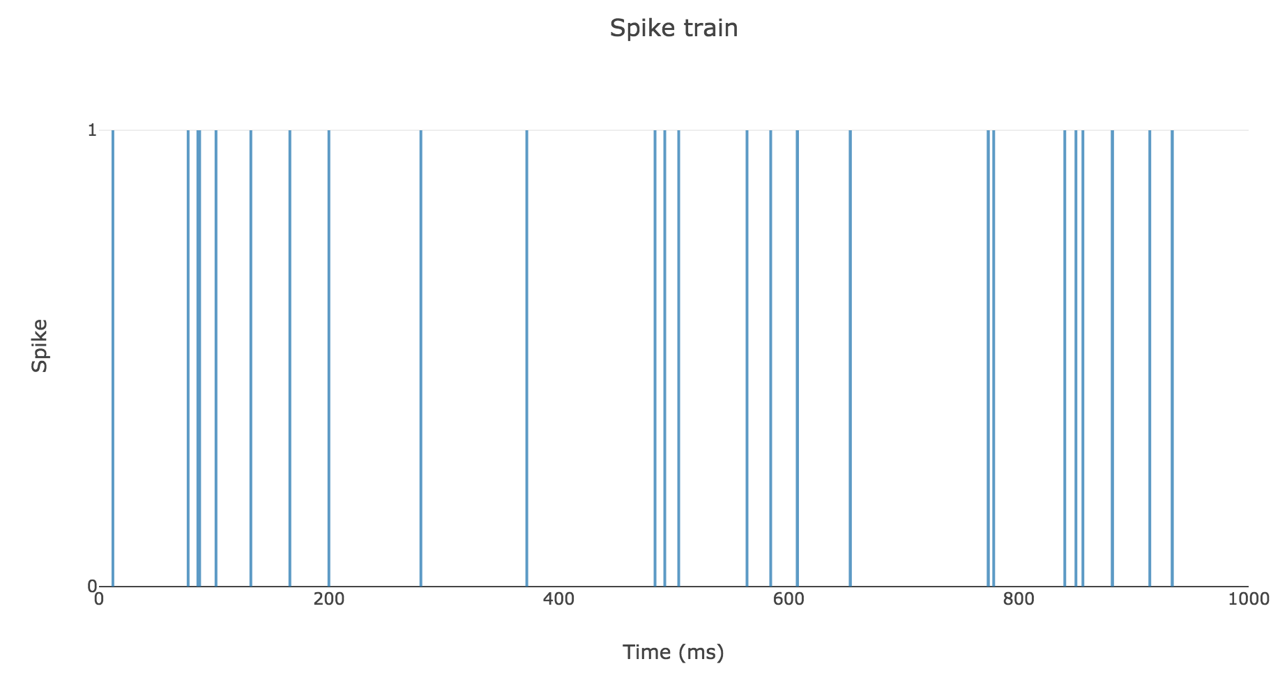
To clarify the time units, let us set

• $Δt ≝ 2 \text{ ms}$
• $T = 1 \text{ s}$
• $r = 25 \text{ spikes/sec}$

Then here is an example of a spike train:

Figure b. - Spike train with a $25 \text{ spikes/sec}$ average rate over $1 \text{ sec}$

2. Spike counts & Interspike intervals

Now, informative features can be extracted from each spike train, such as:

• its total number of spikes (which gives a global information about the spike train, but have us overlook the time step at which each spike occurred)
• the interspike intervals (which give us local clues on the contrary, but encompass the time-related information we lost with the spike counts only)

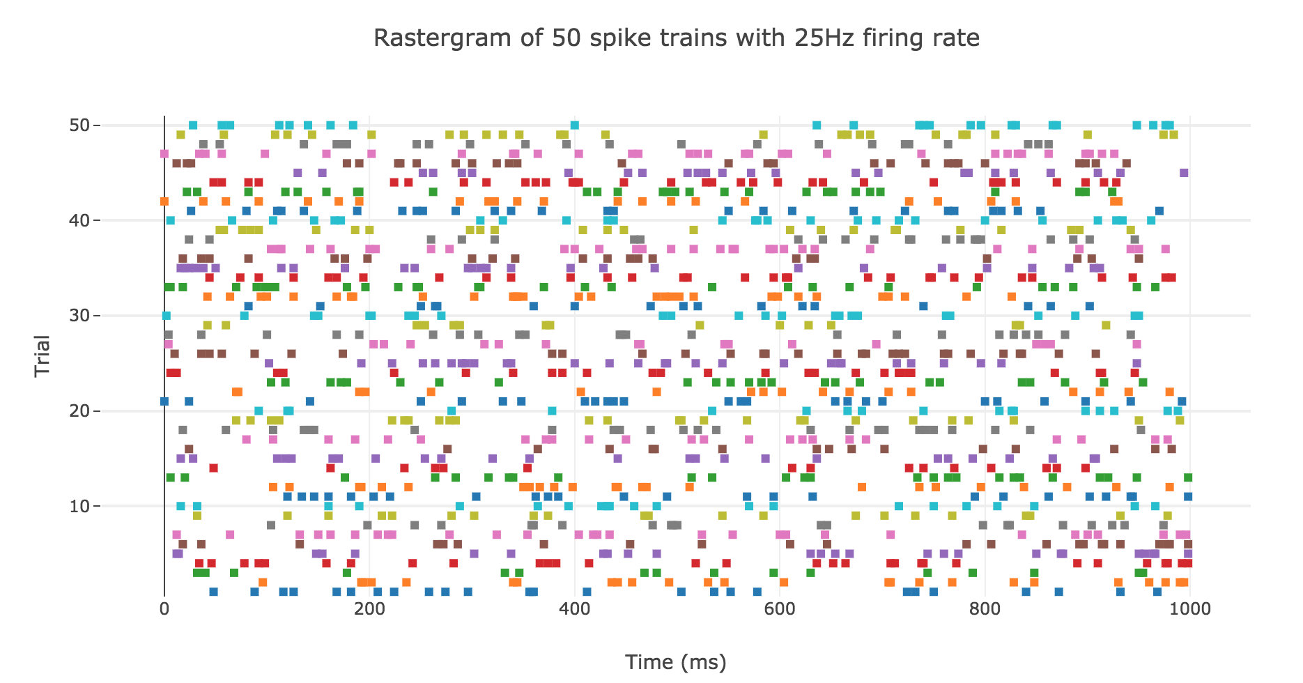
A natural question to ask ourselves is: what is their distribution? To this end, let us generate $N ≝ 200$ spike trains with firing rate $r ≝ 25 \text{ Hz}$.

Here is the rastergram of $50$ of them:

Figure c.1. - Rastergram of $50$ spike trains with a $25 \text{ Hz}$ firing rate

Spike counts

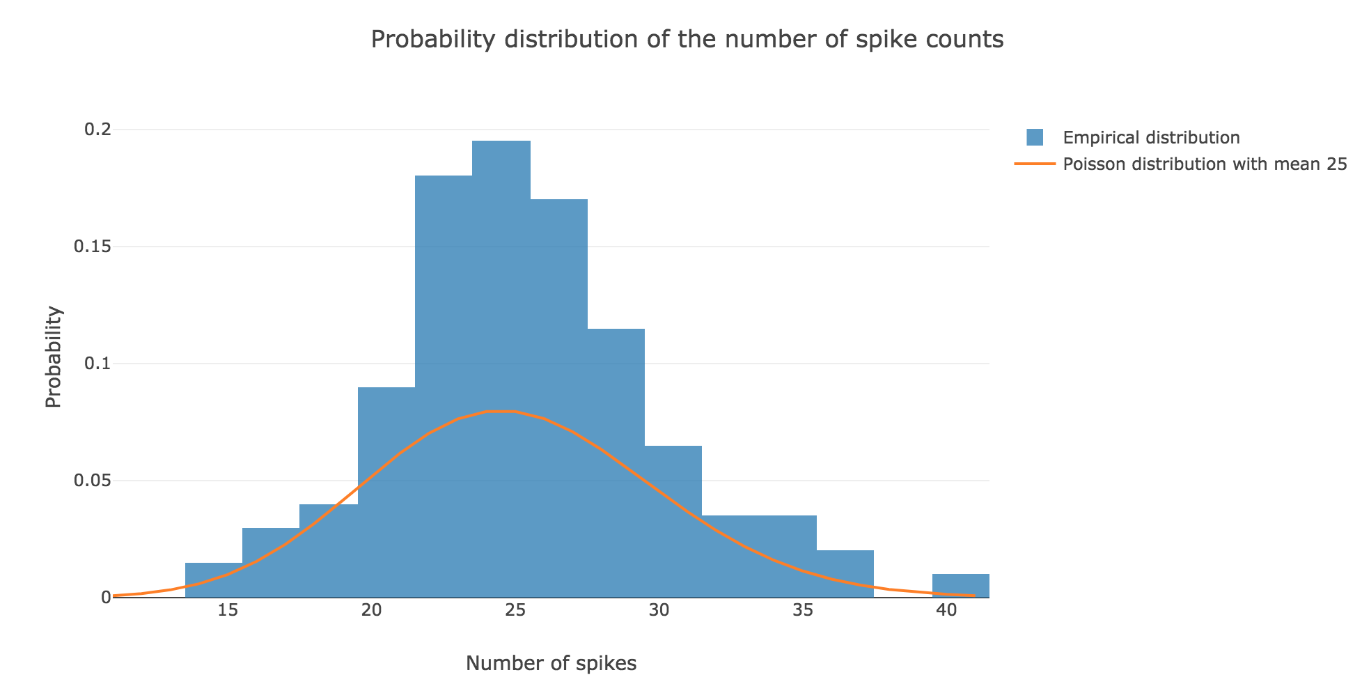
Here is the spike count histogram of all of these $200$ spike trains:

Figure c.2. - Histogram of spike counts for the $N ≝ 200$ spike trains with firing rate $r ≝ 25 \text{ Hz}$

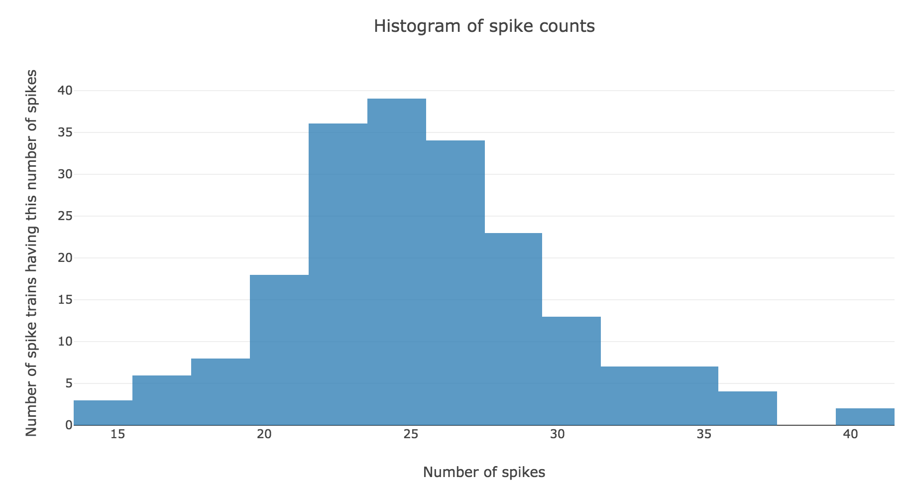
We claim that spike counts are following a Poisson distribution of mean $rT ≝ 25$ (spikes), which may not seem obvious at first sight with so few spike trains:

Figure c.3. - Comparison of the empirical distribution of $N ≝ 200$ spike counts (with firing rate $r ≝ 25 \text{ Hz}$) and the Poisson distribution of mean $rT ≝ 25 \text{ spikes}$

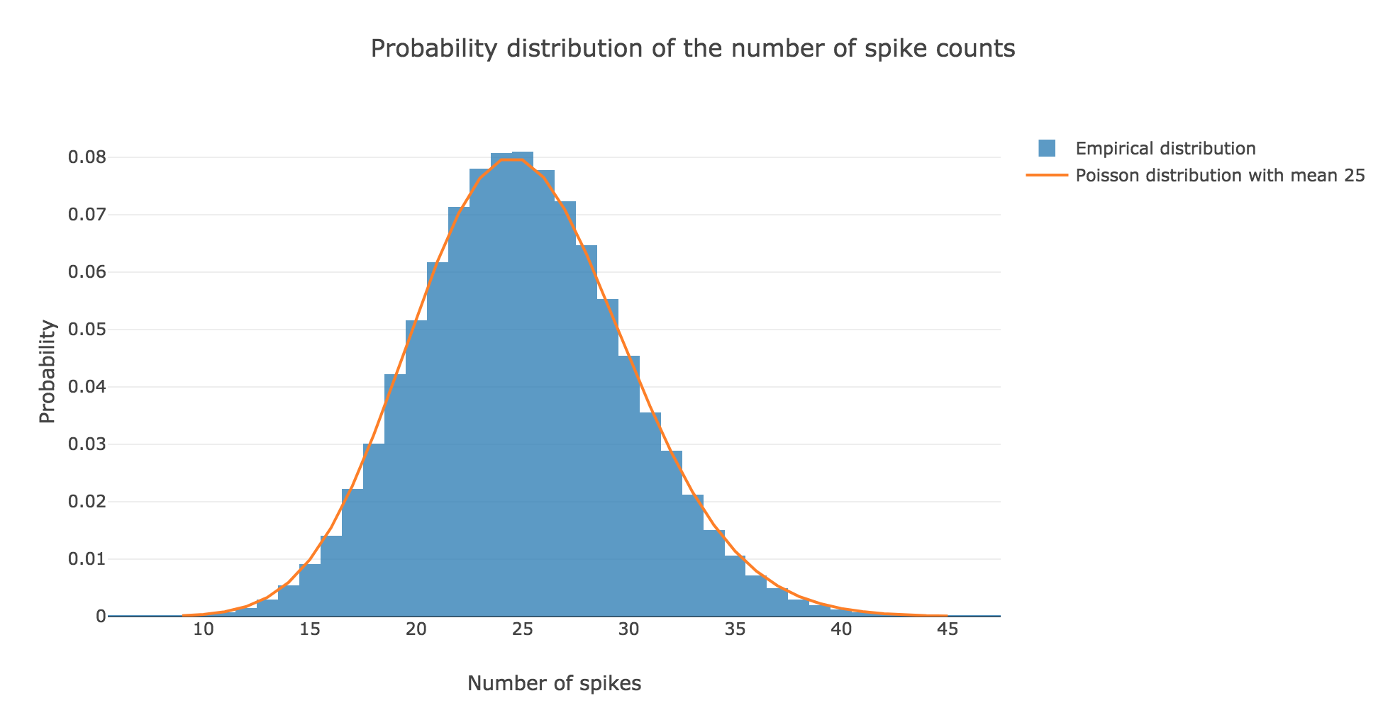
However, it becomes more apparent when the number $N$ of spike trains is increased. For $N ≝ 100000$ for instance:

Figure c.4. - Histogram of spike counts for the $N ≝ 100000$ spike trains with firing rate $r ≝ 25 \text{ Hz}$

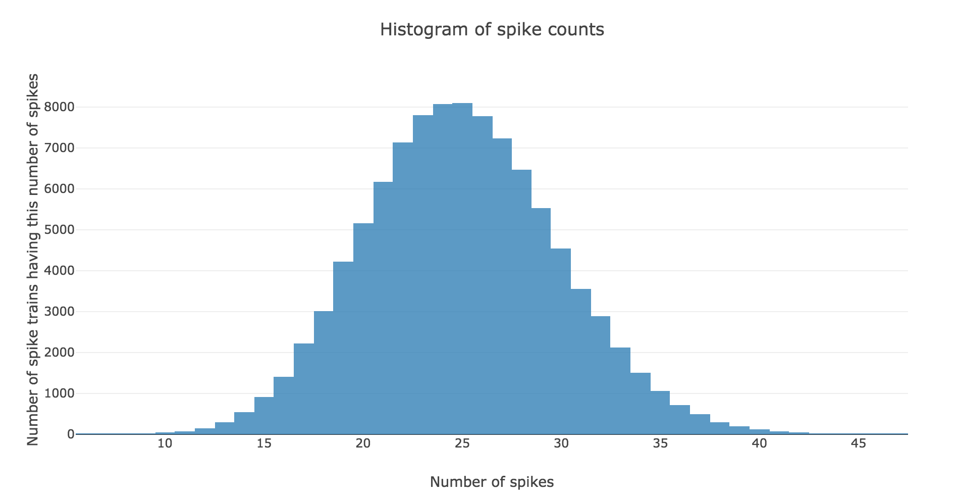
the spike counts distribution matches very well the Poisson one:

Figure c.5. - Comparison of the empirical distribution of $N ≝ 100000$ spike counts (with firing rate $r ≝ 25 \text{ Hz}$) and the Poisson distribution of mean $rT ≝ 25 \text{ spikes}$

This can be explained theoretically: the assumptions stated in the introduction make the Poisson distribution perfectly suited to model the spike counts distribution. More precisely: by definition, the random variable $X$ counting the number of spikes is binomial:

\[X ≝ \sum\limits_{ n=0 }^{M-1} \underbrace{X_{nΔt}}_{\; \sim \; ℬ(rΔt)} \; \sim \; ℬ(M, rΔt)\]

as the $X_t$ are independent (by hypothesis) and identically distributed ($∀t, X_t \sim \; ℬ(rΔt)$).

But it is well known that the Poisson distribution $𝒫(\underbrace{M × rΔt}_{= \, rT})$ successfully approximates such a binomial distribution provided that $M$ is large enough and $rΔt$ is small enough. Here:

• $M ≝ T/Δt = \frac{1000}{2} = 500$
• $rΔt = 25 × 2 \cdot 10^{-3} = 0.05$

which makes the Poisson distribution $𝒫(rT)$, i.e. $𝒫(25)$, perfectly suited to approximate the binomial distribution $ℬ(M, rΔt)$!

Interspike intervals

Here is the interspike interval histogram of $200$ spike trains with firing rate $r ≝ 25 \text{ Hz}$:

Figure d. - Interspike interval histogram of the $N ≝ 200$ spike trains with firing rate $r ≝ 25 \text{ Hz}$

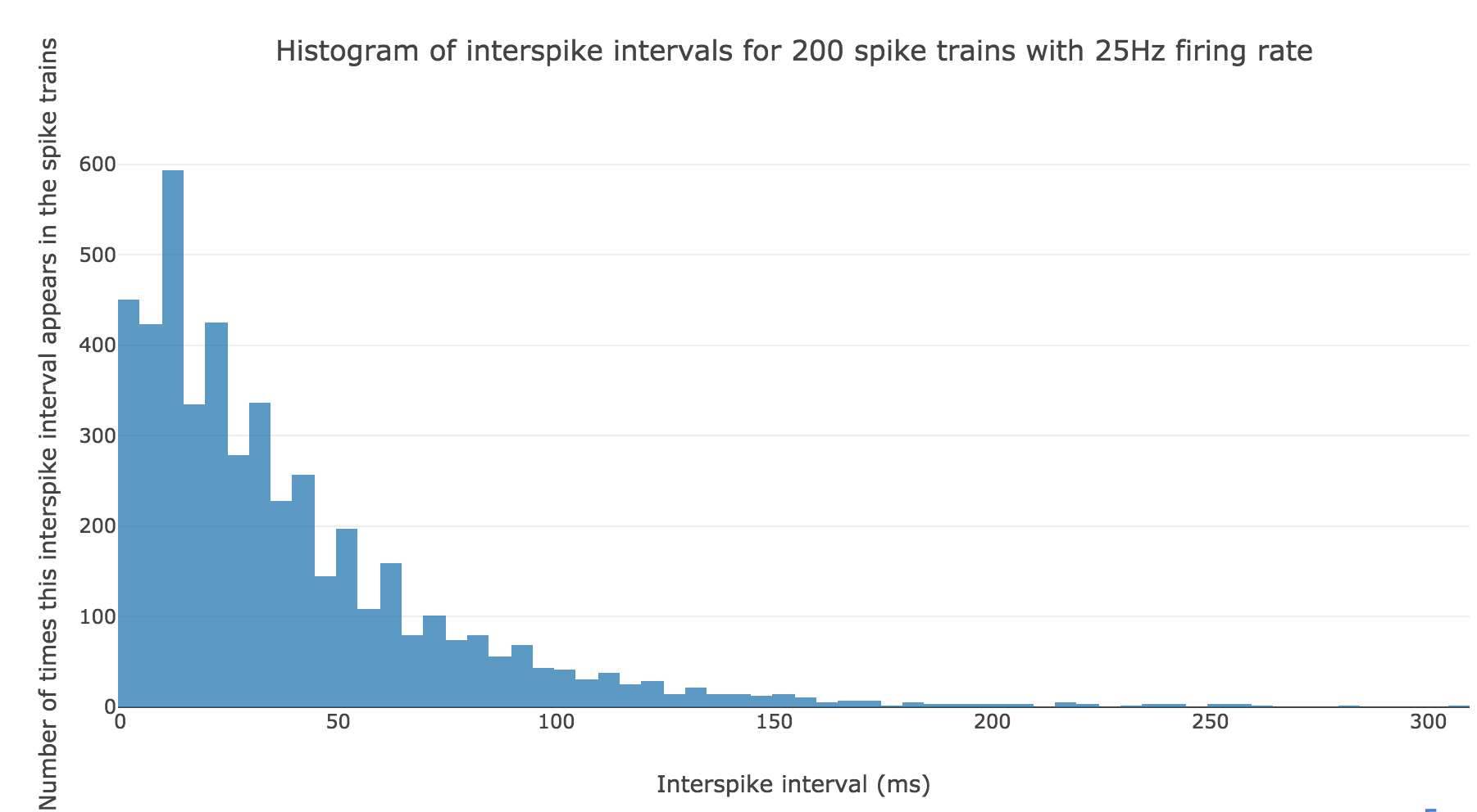
From a theoretical standpoint: if we denote by $Y$ the random variable whose outcome is the length of an interspike interval, in compliance with the assumptions in the introduction, it comes that:

\[\begin{cases} ∀t ≤ 0, \quad P(Y > t) = 1 \\ ∀t > 0, \quad P(Y > t) = (1 - rΔt)^{t/Δt} = \exp\left(\frac{t}{Δt} \ln(1 - rΔt)\right) = \exp\left(- t \, \frac{\ln\left(\frac{1}{1 - rΔt}\right)}{Δt}\right) \end{cases}\]

So:

\[\begin{cases} ∀t ≤ 0, \quad P(Y ≤ t) = 0 \\ ∀t > 0, \quad P(Y ≤ t) = 1 - \exp\left(- t \, \ln\left(\frac{1}{1 - rΔt}\right)/Δt\right) \end{cases}\]

Therefore, by definition of its cumulative distribution function, the interspike interval variable $Y$ follows an exponential distribution of rate $\ln\left(\frac{1}{1 - rΔt}\right)/Δt$

PROBLEM 2: Analysis of spike train

Link of the iPython notebook for the code

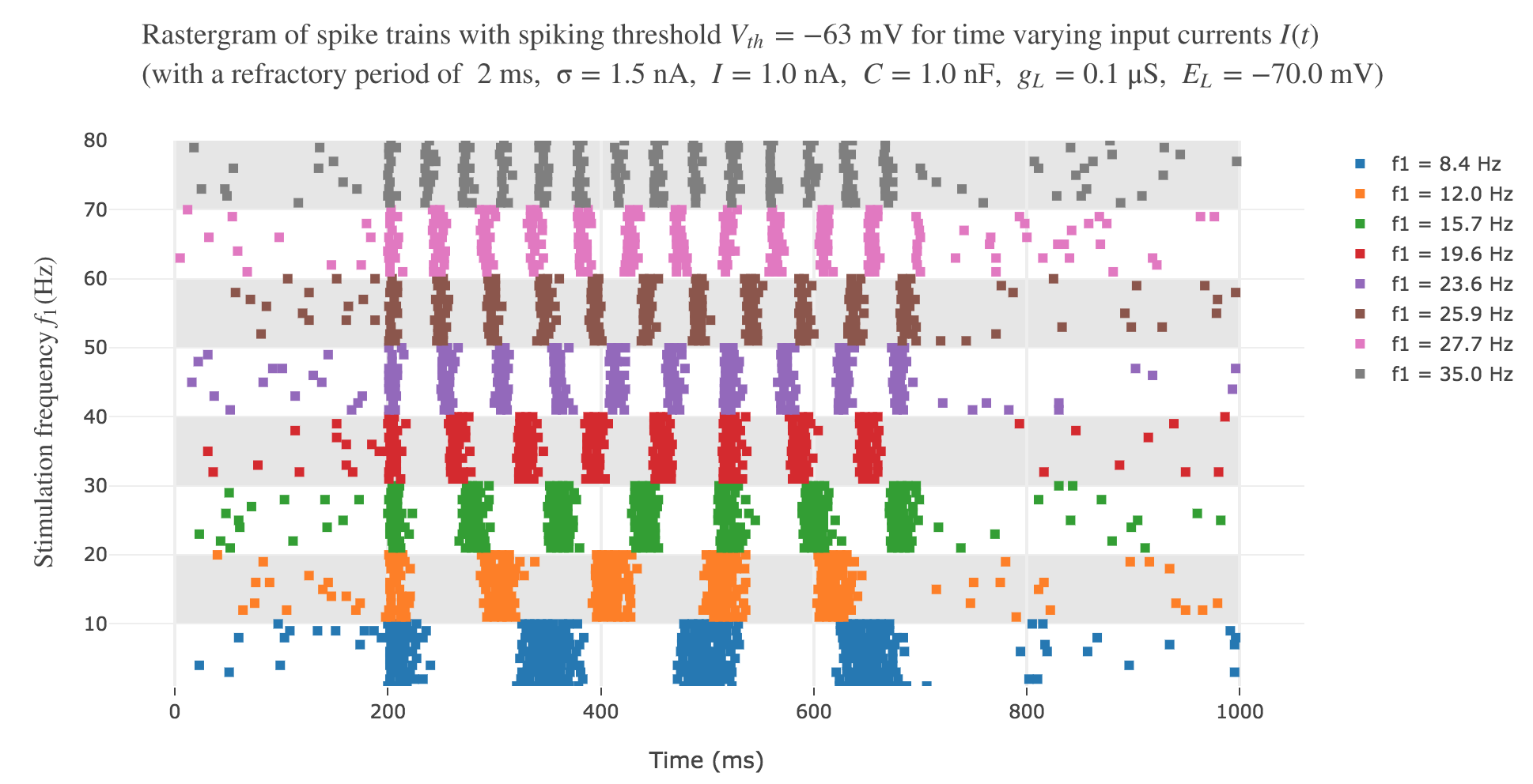
One records and analyses several spike trains from a single neuron in the primary somatosensory cortex of a monkey experiencing a vibratory stimulus on the fingertip, for different vibration frequencies $f_1 ∈ \lbrace 8.4, 12, 15.7, 19.6, 23.6, 25.9, 27.7, 35\rbrace \text{ Hz}$. The simulation is conducted between $200$ and $700$ msec.

Figure a. - Rastergram of the spike trains for the first $8.4$ Hz vibration frequency

Figure b. - Rastergram of the spike trains for various vibration frequencies

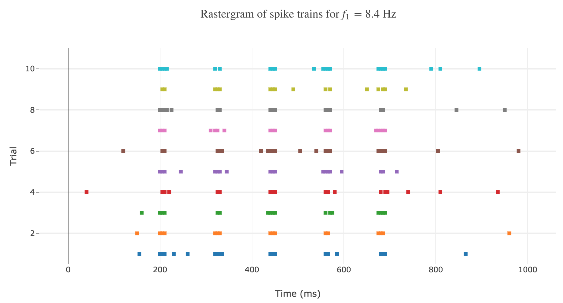
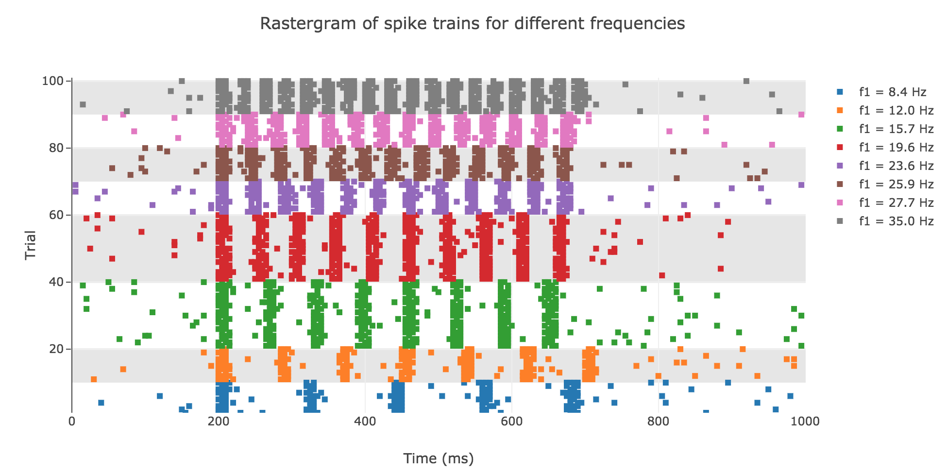
As shown in Figure a. and Figure b., the spikes within the simulation period (between $200$ and $700$ msec):

• seem to be periodically spaced for a given frequency $f_1$
• are more and more numerous as the frequency increases

and even more: the number of spikes seem to depend linearly on the vibration frequency.

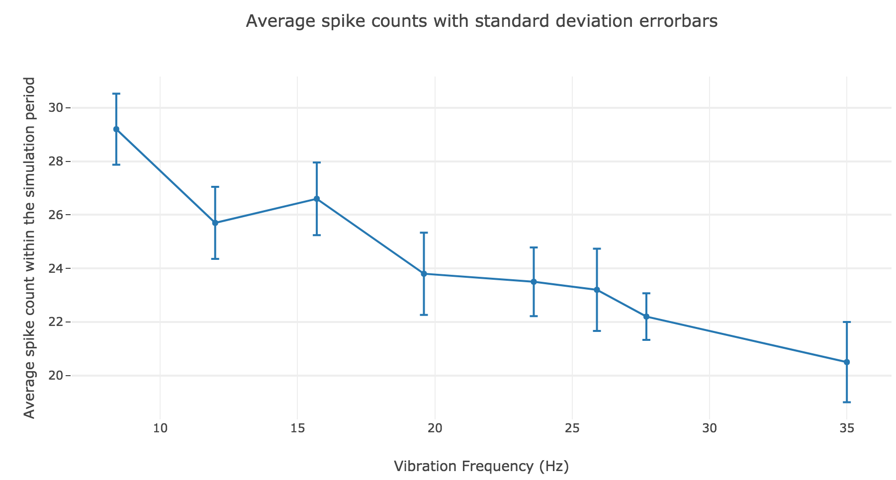
The latter observation is backed up by the shape of the average spike count, plotted as a function of the vibration frequency:

Figure c.1. - Average spike count as a function of the vibration frequency with standard deviation errorbars

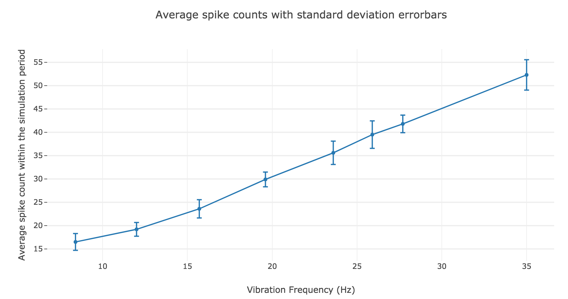
A linear regression of the average spike counts (as a function of the vibration frequency) can me made:

• Linear equation: \(y = 1.39 x + 3.08\)
• Correlation coefficient: $0.997$
• Standard error of the estimate: $0.04$

The very high correlation coefficient and very low standard error of the estimate highlight an almost perfect match!

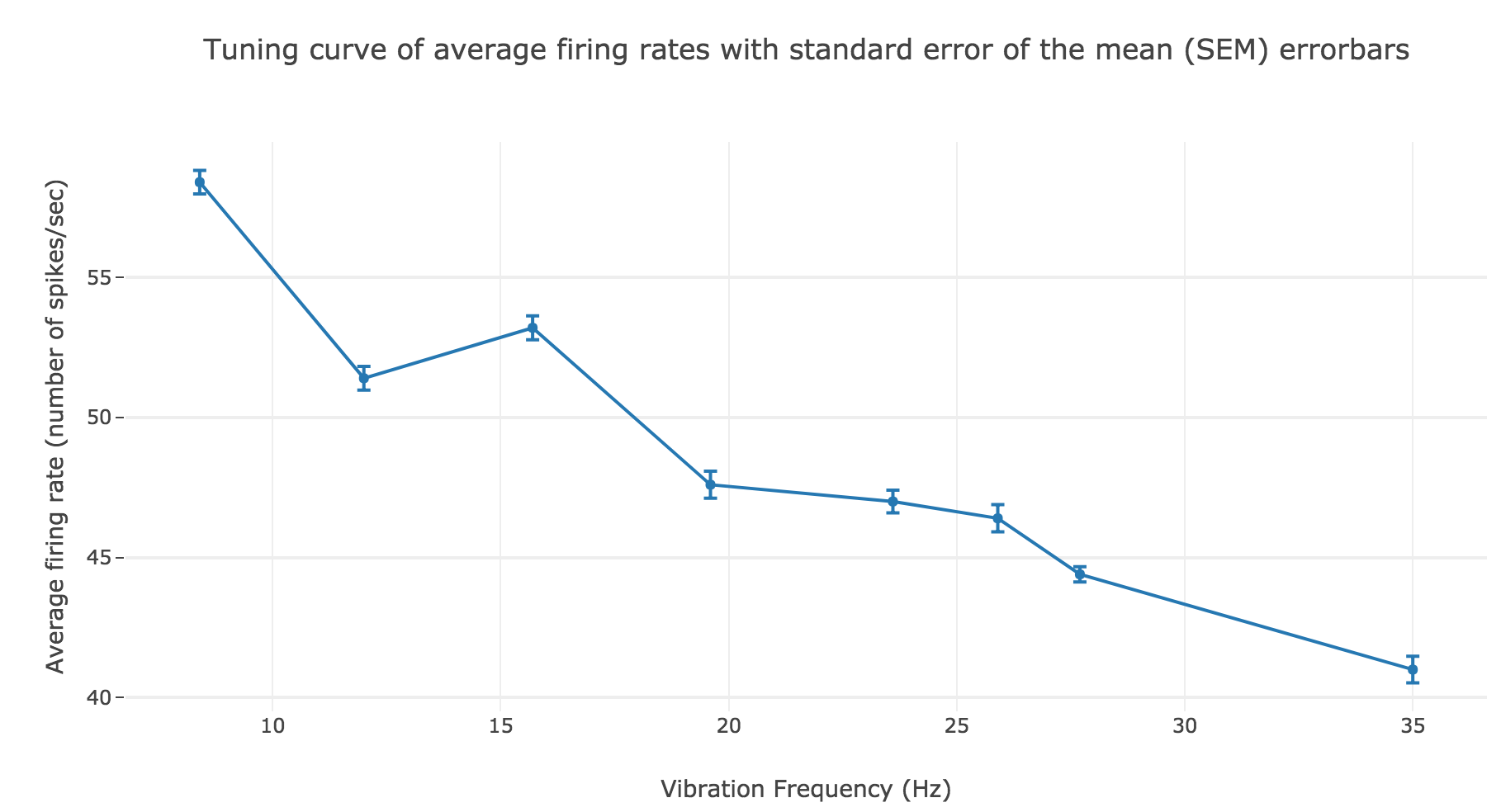
We have similar results for the average firing rate as a function of the vibration frequency:

Figure c.2. - Average firing rate as a function of the vibration frequency with standard error of the mean $SEM = σ/ \sqrt{N}$ errorbars

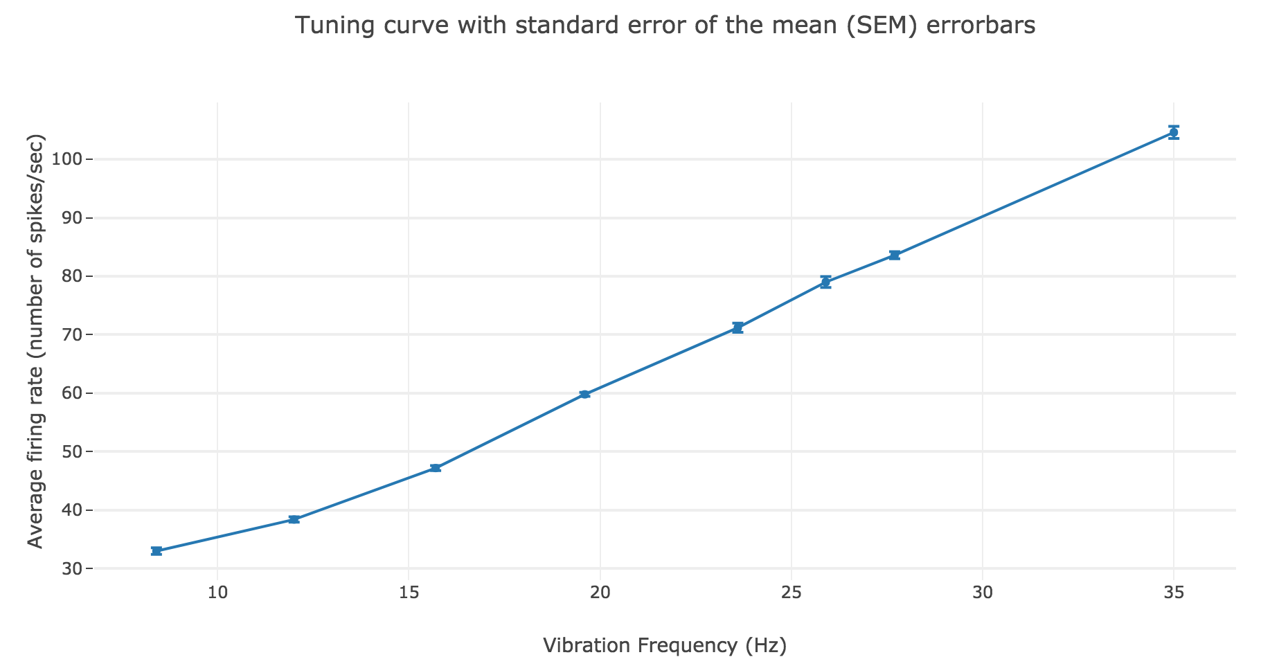
The linear regression yields:

• Linear equation: \(y = 2.78 x + 6.15\)
• Correlation coefficient: $0.997$
• Standard error of the estimate: $0.08$

As a result: the firing rate of the neuron can be regarded as a non-decreasing linear function of the vibration frequency.

PROBLEM 3: Integrate-and-Fire neuron

Link of the iPython notebook for the code

We will now:

• first study the integrate-and-fire model with a constant input current, to acount for the creation of action potential (spikes) in real neurons

• secondly make the input current vary over time, to try to account for the spike trains that were experimentally measured in the primary somatosensory cortex of a monkey experiencing a vibratory stimulus on the finger (cf. the previous problem)

1. Integrate-and-Fire neuron with constant input current

Voltage accross a passive membrane

The voltage across a passive neuron’s membrane when a current $I$ is injected is given by:

\[C \frac{ {\rm d}V}{ {\rm d}t} = g_L (E_L - V(t))+I\]

where

• $C = 1 \text{ nF}$ is the membrane capacitance
• $g_L = 0.1 \text{ μS}$ is the leak conductance of the membrane
• and $E_L = −70 \text{ mV}$ its reversal potential

On top of that, we will set

• $I$ to be equal to $1 \text{ nA}$
• $V(0)$ to be equal to $E_L$

The Euler method yields:

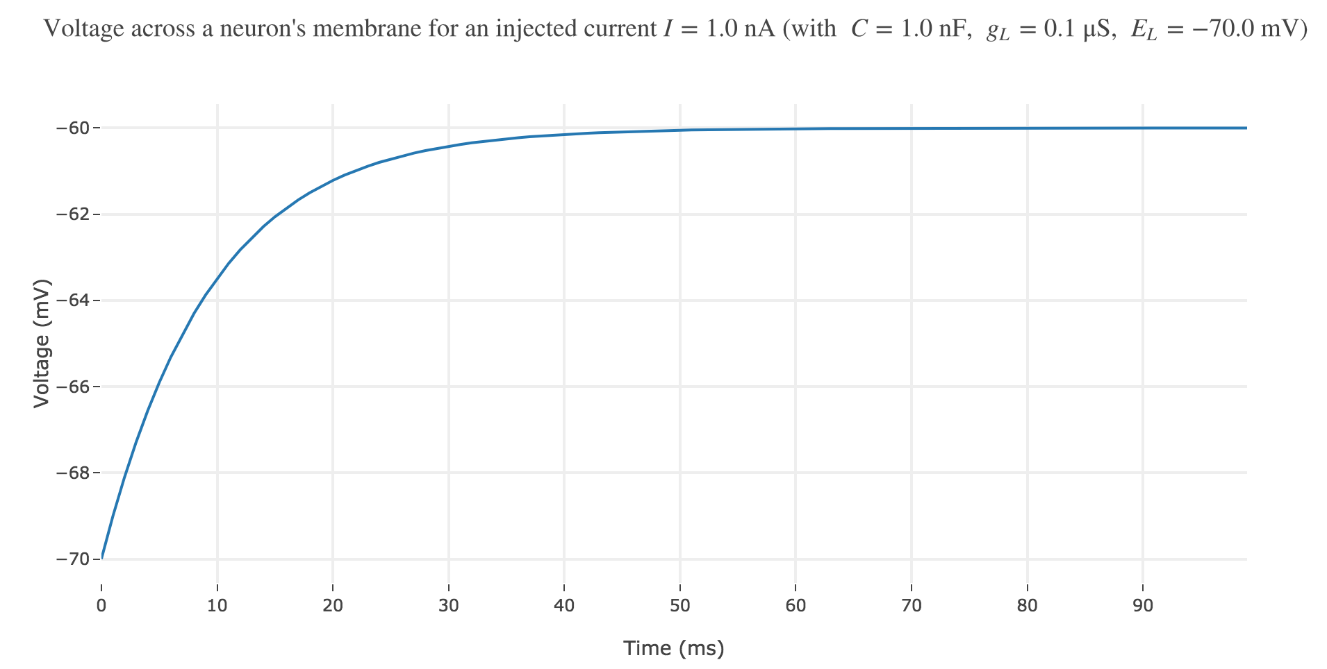
\[\begin{align*} & \; C \frac{ ΔV}{ Δt} = g_L (E_L - V(t))+I\\ ⟺ & \; \frac{ ΔV}{ Δt} = \frac 1 C (g_L (E_L - V(t))+I)\\ ⟺ & \; V(t+Δt) - V(t) = \frac {Δt} C (g_L (E_L - V(t))+I)\\ ⟺ & \; V(t+Δt) = \Big(1- \frac {Δt \cdot g_L} C\Big) V(t) + \frac {Δt \, (g_L \, E_L + I)} C \end{align*}\]

which enables us, by setting $∆t = 1 \text{ ms}$, to plot the voltage until time $t = 100 \text{ ms}$ for instance:

Figure a. - Voltage accross a neuron's passive membrane for an injected current $I=1 \text{ nA}$

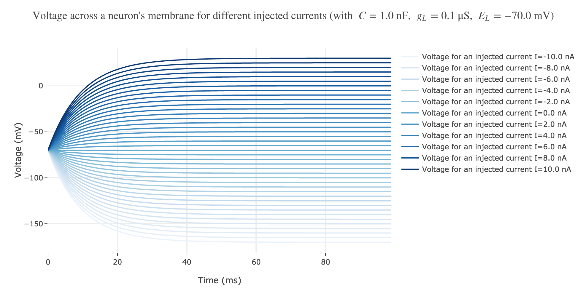
Now, for various current inputs $I$:

Figure b.1. - Voltage accross a neuron's passive membrane for positive different injected currents

Figure b.2. - Voltage accross a neuron's passive membrane for different positive and negative injected currents

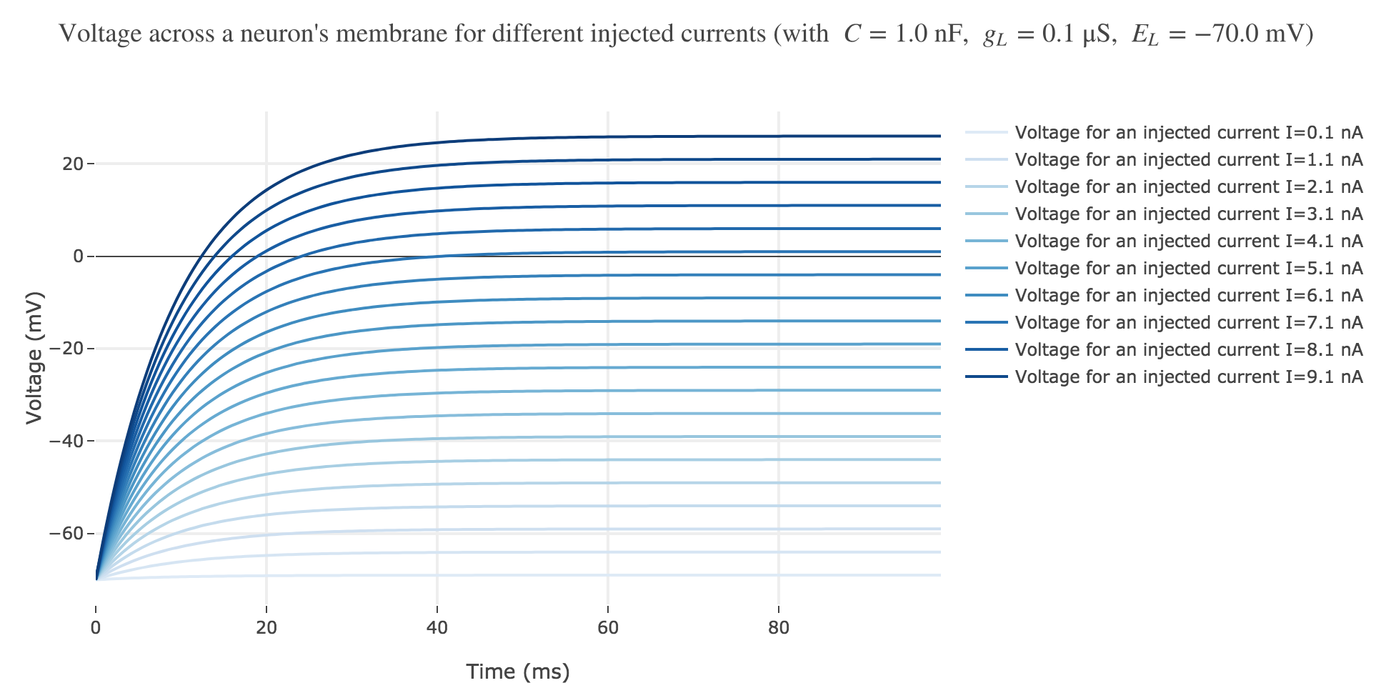
For positive currents: It appears that the voltage accross the passive membrane is a non-decreasing monotonous function of the time (reaching a plateau after $40$ ms in our case) which increases when the input current does so.

For the negative currents: the curves are symmetric to the positive current ones with respect to the $V = E_L$ line.

To be more precise, let us solve for $V$ analytically:

\[\begin{align*} & \; \frac{ {\rm d}V}{ {\rm d}t} = \frac {g_L} C (E_L - V(t))+I/C\\ ⟺ & \; \frac{ {\rm d}V}{ {\rm d}t} + \frac {g_L} C V(t) = \frac {g_L \, E_L +I} C\\ ⟺ & \; \frac{ {\rm d}V}{ {\rm d}t} \, {\rm e}^{\frac {g_L \, t} C} + \frac {g_L} C V(t) \, {\rm e}^{\frac {g_L \, t} C} = \frac {g_L \, E_L +I} C \, {\rm e}^{\frac {g_L \, t} C}\\ ⟺ & \; \frac{ {\rm d}}{ {\rm d}t} \left[V(t) \, {\rm e}^{\frac {g_L \, t} C}\right] = \frac {g_L \, E_L +I} C \, {\rm e}^{\frac {g_L \, t} C}\\ ⟺ & \; V(t) \, {\rm e}^{\frac {g_L \, t} C} = \frac C {g_L} \frac {g_L \, E_L +I} C \, {\rm e}^{\frac {g_L \, t} C} + \text{const}\\ ⟺ & \; V(t) \, {\rm e}^{\frac {g_L \, t} C} = \left(E_L + \frac I {g_L}\right) \, {\rm e}^{\frac {g_L \, t} C} + \text{const}\\ ⟺ & \; V(t) \, = \left(E_L + \frac I {g_L}\right) + \text{const} × {\rm e}^{-\frac {g_L \, t} C}\\ \end{align*}\]

And with $V(0) = E_L$:

\[∀t ≥0, \quad V(t) \, = E_L + \frac I {g_L}\left(1-{\rm e}^{-\frac {g_L \, t} C}\right)\]

The symmetry with respect to the $V = E_L$ between negative and positive current curves is clearly seen in this analytical expression.

Figure c. - Voltage accross a neuron's membrane: Comparison between the numerical solution and the exact one

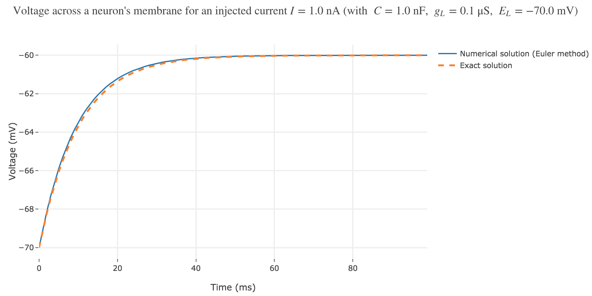
As seen in Figure c. the numerical solution resulting from the Euler method and the exact one closely match.

So, on the whole:

• $V$ starts at $E_L$
• and then increases monotonously until $E_L + I/g_L$ (so the higher the input current, the higher the voltage, as examplified in Figure b)
• the characteristic time constant thereof is $C/g_L = 10 \text{ ms}$

• the derivative of $V$:

  \[\frac{ {\rm d}V}{ {\rm d}t} ≝ \frac{I}{C} \, {\rm e}^{-\frac {g_L \, t} C}\]

  is positively proportional to $I$: the higher the input current, the steeper the increase of $V$.

Action-potential-generating mechanism

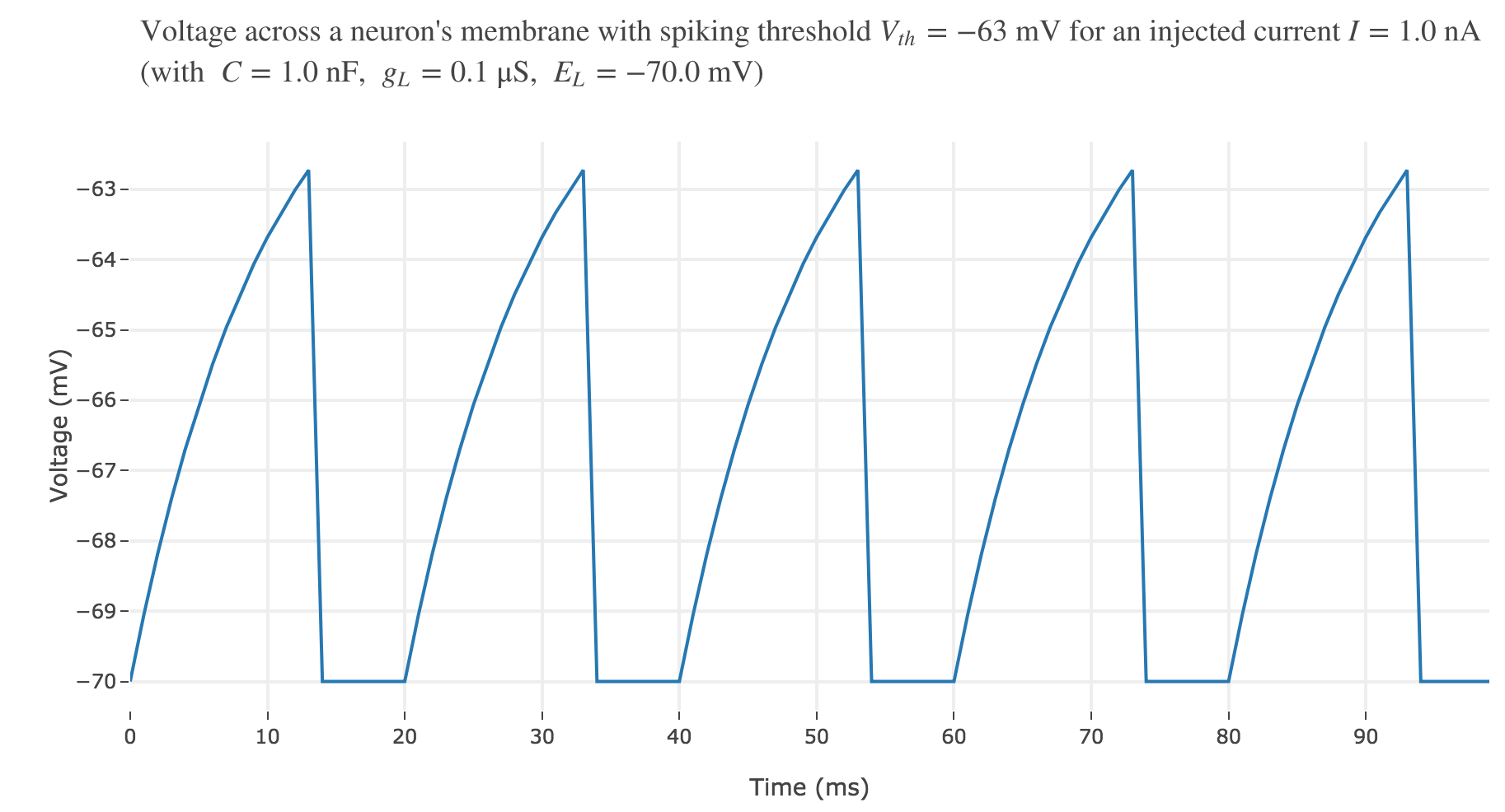
To account for spike generation, let us assume that the neuron fires each time $V$ gets greater than a threshold $V_{th}$, after which the membrane voltage is reset to its initial value $E_L$. Let us set $V_{th} ≝ −63 \text{ mV}$:

Figure d.1. - Voltage accross a neuron's membrane with spiking threshold $V_{th} ≝ −63 \text{ mV}$ and an injected current of $1$ nA.

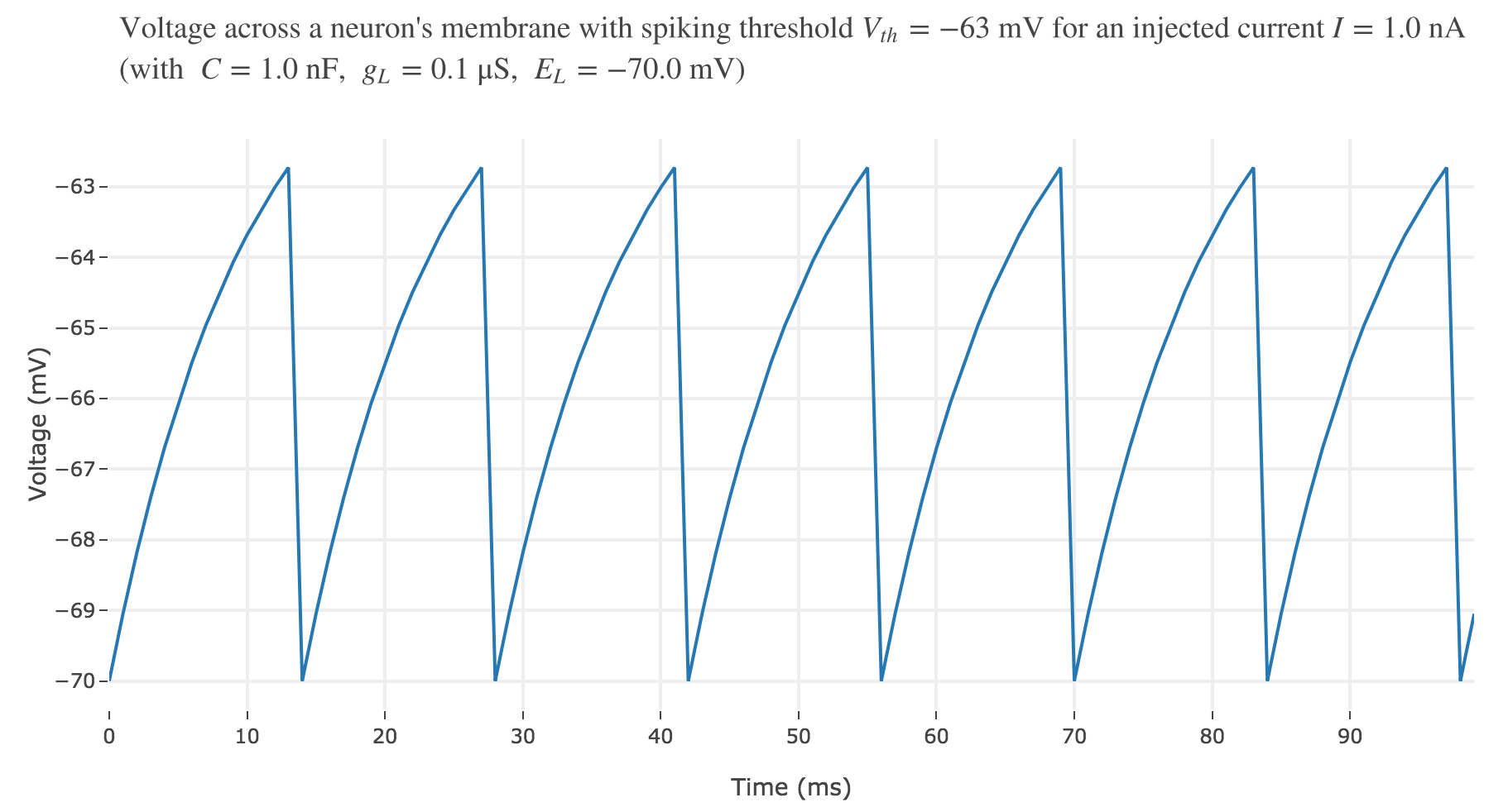
For an input current of $1$ nA, we get $7$ spikes within the first $100$ ms. Let us investigate how the number of spikes varies with the input current:

Figure d.2. - Voltage accross a neuron's membrane with spiking threshold $V_{th} ≝ −63 \text{ mV}$ and different injected currents $≤ 0.75$ nA

Figure d.3. - Voltage accross a neuron's membrane with spiking threshold $V_{th} ≝ −63 \text{ mV}$ and injected currents $0.8$ and $1.3$ nA

Figure d.4. - Voltage accross a neuron's membrane with spiking threshold $V_{th} ≝ −63 \text{ mV}$ and injected currents $1.3$ and $1.8$ nA

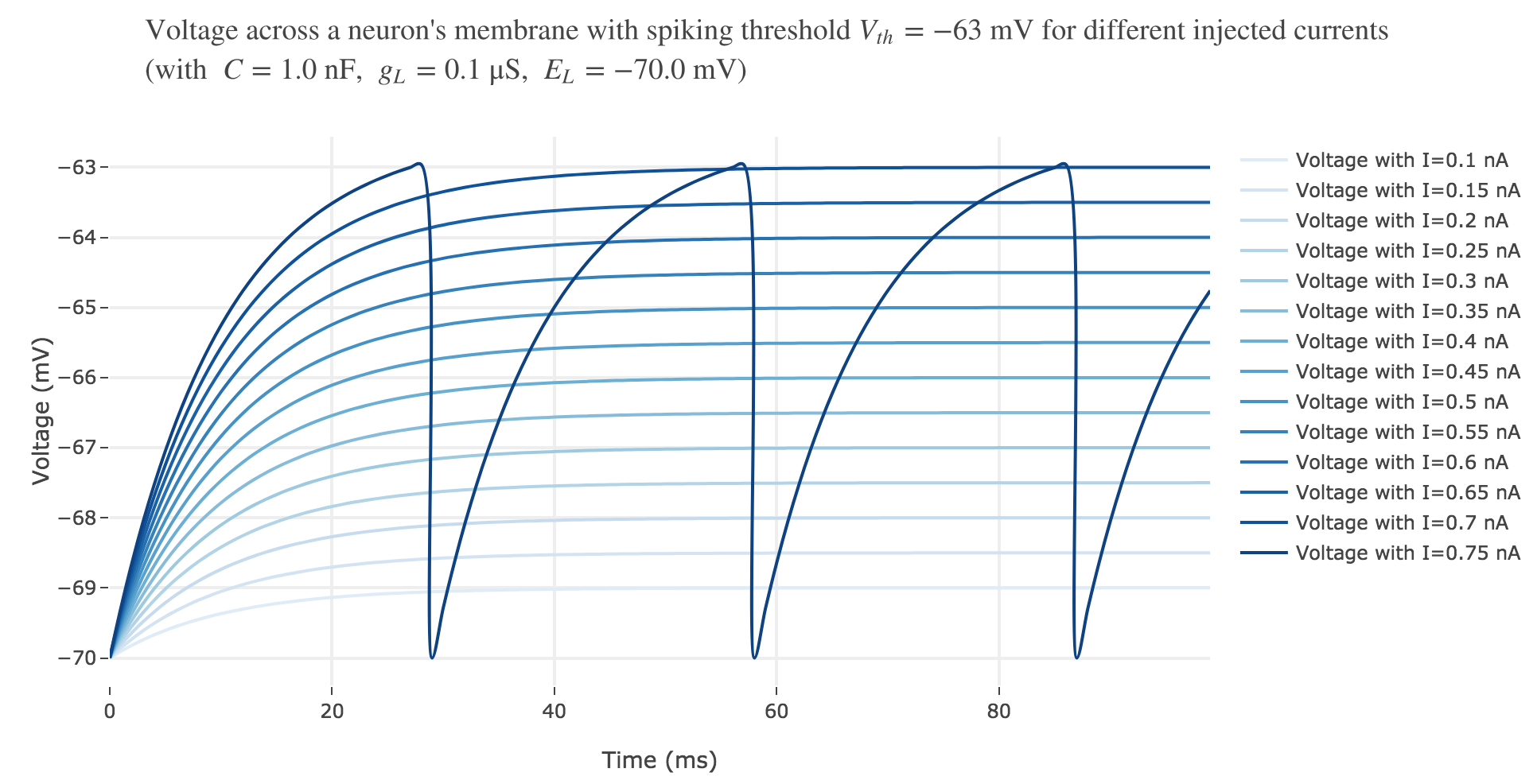
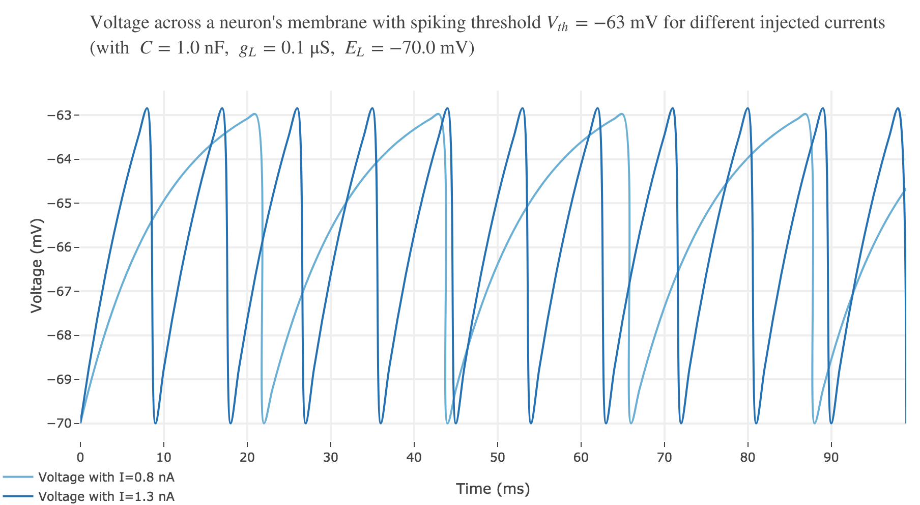
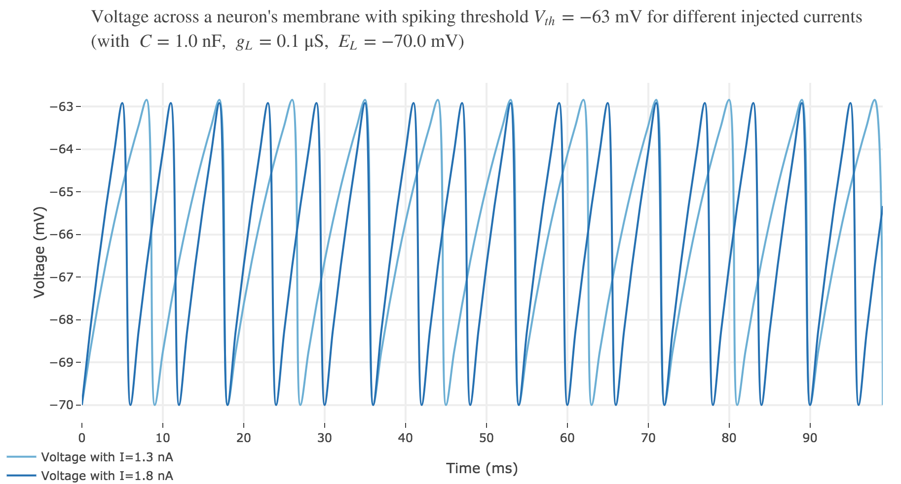
For $I ≥ 0.75$ nA: The higher the input current, the steeper the increase of $V$ (as shown before) and hence the the faster $V$ reaches the threshold: so, as expected, we observe that the higher the input current, the higher the number of spikes within $100$ ms.

But for $I ≤ 0.7$ nA, no spike is fired. Indeed, the precise input current value at which the neuron start firing can be computed analytically:

\[\begin{align*} & \; ∃t; \; V(t) \, \overset{\text{eventually}}{>} V_{th}\\ ⟺ & \; \lim\limits_{t \to +∞} V(t) > V_{th} &&\text{ (as } V \text{ is non-decreasing)}\\ ⟺ & \; E_L + \frac I {g_L} > V_{th}\\ ⟺ & \; I > g_L (V_{th} - E_L) \end{align*}\]

As it happens, with with $E_L ≝ -70 \text{ mV}$ and $V_{th} = -63 \text{ mV}$:

\[∃ t; \quad V(t) \, \overset{\text{eventually}}{>} V_{th} ⟺ I > 0.7 \text{ nA}\]

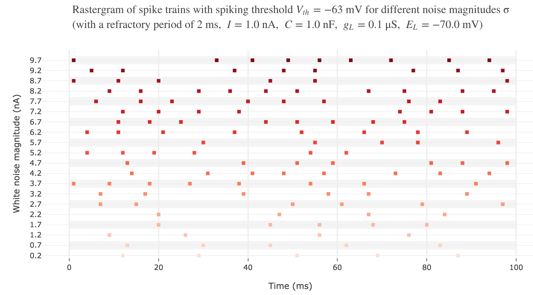
Let us plot a rastergram of the spike trains for various injected currents, so as to to see more easily how the number of spikes is impacted:

Figure d.5. - Rastergram of spike trains with spiking threshold $V_{th} ≝ −63 \text{ mV}$ for various injected currents

For $I ≥ 7.8$ nA, the number of spikes reaches its maximum value of $49$ spikes within $100$ ms.

To make it even more clear, let us plot the tuning curve of this neuron (i.e. the number of spikes within $100 \text{ ms}$ depending on the input current $I$):

Figure d.6. - Number of spikes within $100 \text{ ms}$ as a function of the input current $I$

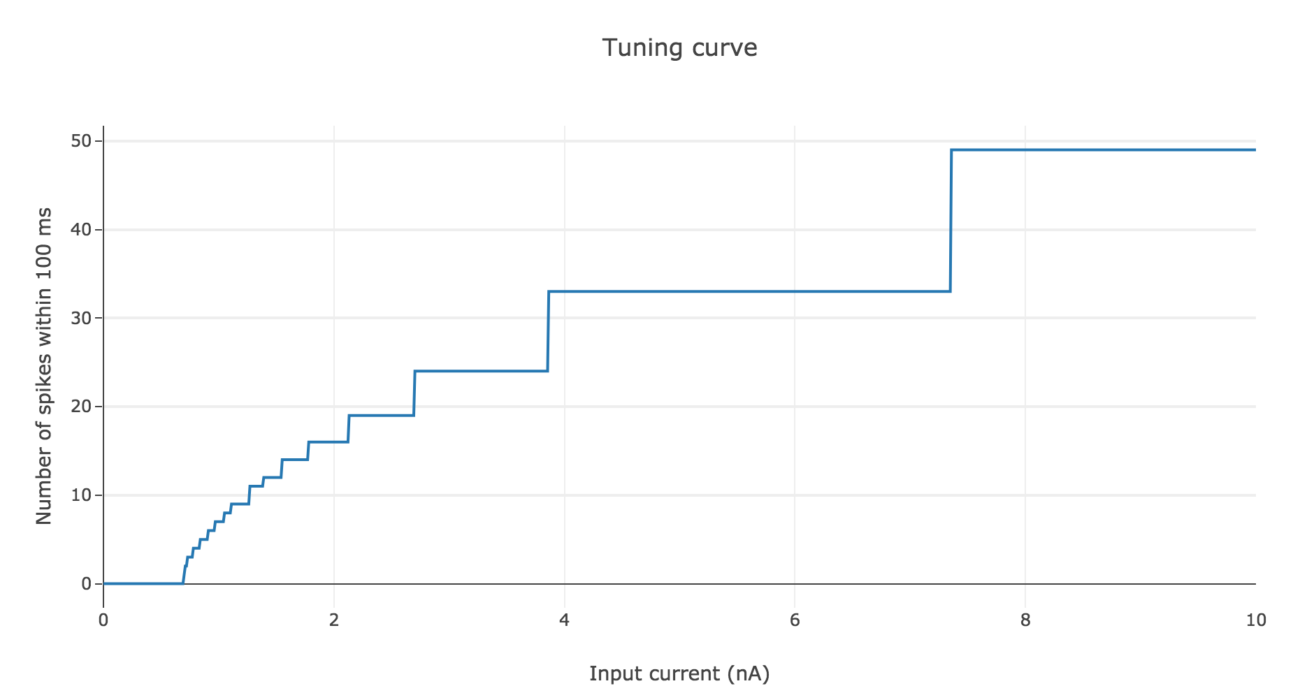
As shown before, the current threshold at which the neuron starts firing is

\[I_{th} ≝ g_L (V_{th} - E_L)\]

This makes sense intuitively:

• the higher the difference $V_{th} - E_L$, the more the voltage $V$ has to increase to reach $V_{th}$ within $100 \text{ ms}$, and we saw previously that it requires a higher input current $I$

• the higher the leak conductance $g_L$ of the membrane, the lower the voltage $V$ by Ohm’s law (as $V$ is inversely proportional to the conductance), and the higher the input current is required to be, to compensate

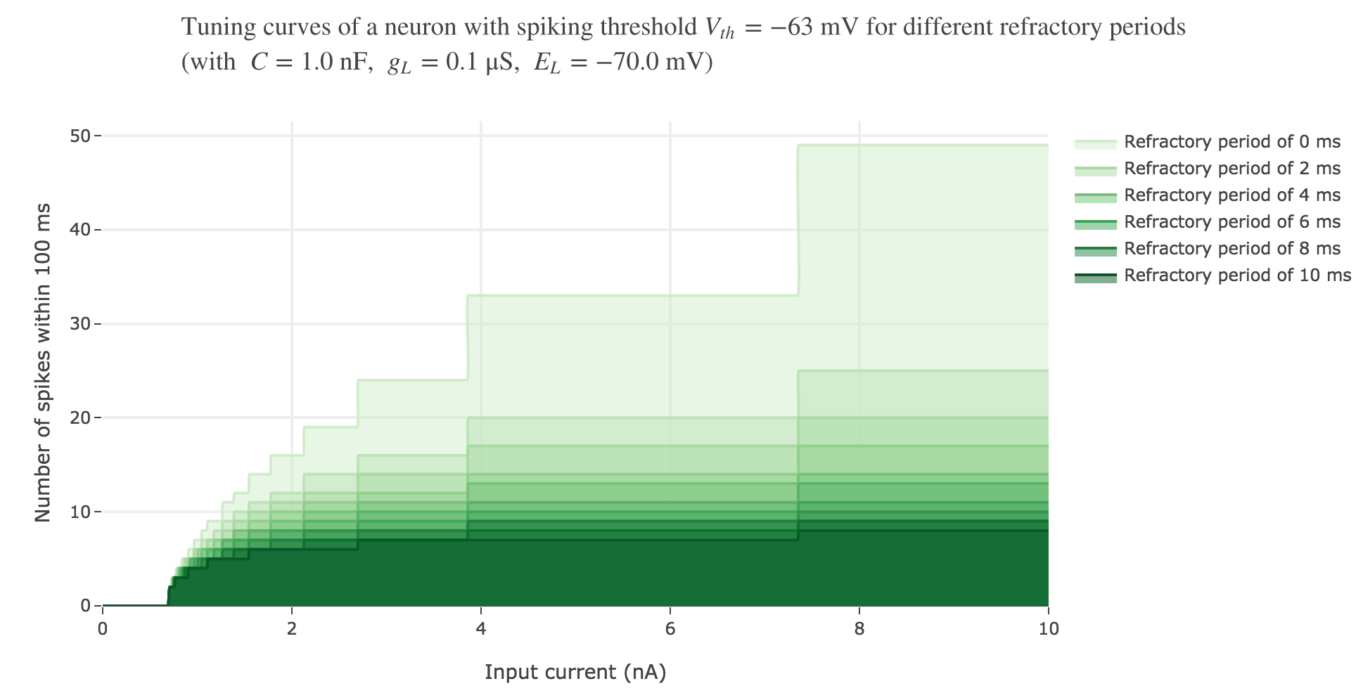
Refractory period

Whenever the neuron depolarize until the voltage hits the threshold: it fires, then the voltage is reinitialized at $E_L$, but it can be shown experimentally that the voltage doesn’t increase right away after having been reset: for a fixed time span (the refractory period), the voltage remains constant, then at the end of the refractory period it depolarizes again.

We can take into account this refractory period in our model:

Figure f.1. - Voltage accross a neuron's membrane with spiking threshold $V_{th} ≝ −63 \text{ mV}$ and a $1$ nA input current, having a $5 \text{ msec}$ refractory period.

On goes from $7$ spikes (before) to $5$ ones within the first $100$ ms, with a $5$ ms refractory period.

As expected: the higher the refractory period, the less spike the neuron fires within the same time span.

Figure f.2. - Number of spikes within $100 \text{ ms}$ as a function of the input current $I$ for different refractory periods.

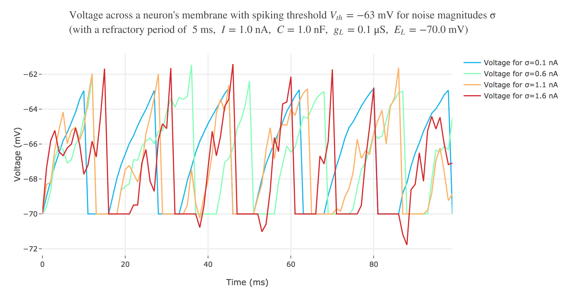
With a white noise term

A more realistic model would take into account part of the noise there is in reality. A more noisy voltage accross a neuron’s passive membrane could be given by:

\[C \frac{ {\rm d}V}{ {\rm d}t} = g_L (E_L - V(t))+ I + ση(t)\]

where $σ$ is the noise magnitude and $η \sim 𝒩(0, 1)$. The choice of a Gaussian distribution is accounted for by the central limit theorem, since the noise can be thought of as a sum of many independent indentically distributed processes.

The Euler method yields:

\[C (V(t+ Δt) - V(t)) = g_L (E_L - V(t)) Δt + I Δt + σ \sqrt{Δt} \, η(t)\]

Thus:

\[V(t+Δt) = \Big(1- \frac {Δt \cdot g_L} C\Big) V(t) + \frac {Δt \, (g_L \, E_L + I)} C + \frac {σ \sqrt{Δt} \, η(t)} C\]

The $\sqrt{Δt}$ stems from the fact that

\[\sqrt{Δt} \, η(t) \sim 𝒩(0, Δt)\]

so that the noise magnitude amounts to $Δt$ when adding a $Δt$ time step.

The white noise term makes it look more realistic:

Figure g.1. - Voltage accross a neuron's membrane with spiking threshold $−63 \text{ mV}$, a $1$ nA input current and a $5 \text{ msec}$ refractory period, for various noise magnitudes

Figure g.2. - Rastergram of spike trains with spiking threshold $−63 \text{ mV}$,a $1$ nA input current and a $5 \text{ msec}$ refractory period, for various noise magnitudes

2. Integrate-and-Fire neuron with time-varying input current to match experimental data

Finally, let us try to model the experminental spike trains generated by a given neuron in the primary somatosensory cortex of a monkey subject to a vibratory stimulus on the finger (as seen in the previous problem).

Figure h.1. - Rastergram of the experimental spike trains for various vibration frequencies

To do so, a constant input current will not be enough, as shown in Figure g.2.: the rastergram is not likely to match what is observed experimentally. And above all, the vibration frequency $f_1$ has not even been taken into account so far, which cannot but lead us to fail to model the experimental spike trains, as we showed that there is a linear relationship between the average spike counts/firing rates and the vibration frequencies.

Looking at the experimental spike trains, we observed in the previous problem that the spikes seemed to occur periodically within the simulation time span (between $200$ and $700$ ms): the higher the vibration frequency, the smaller the interspike period.

This suggests a sinusoidal input current whose frequency is a multiple of the vibration frequency, modulated by an envelope that decays out of the simulation period.

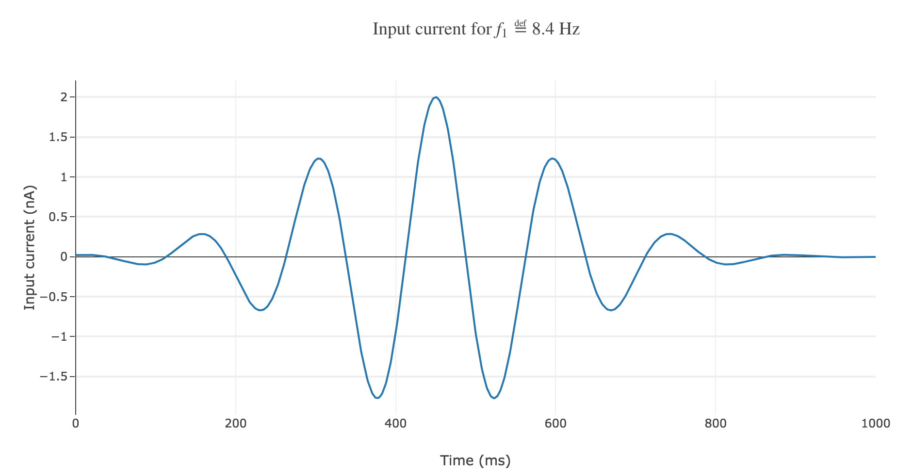
Gaussian envelope

With a Gaussian envelope, the time-varying input current

\[I(t) \propto \exp\left(-\frac{(t - μ)^2}{2 s^2}\right) \cos(f_1 (t-μ)/200)\]

where $μ = 450 \text{ ms}, \; s = 150 \text{ ms}$, could look like this:

Figure h.2. - Sinusoidal input current with a Gaussian envelope

It leads to the following rastergram:

Figure h.3. - Rastergram of artifical spike trains induced by a sinusoidal input current modulated by a Gaussian envelope, for various vibration frequencies

which is not satisfying, with regard to the experimental one.

Heaviside envelope

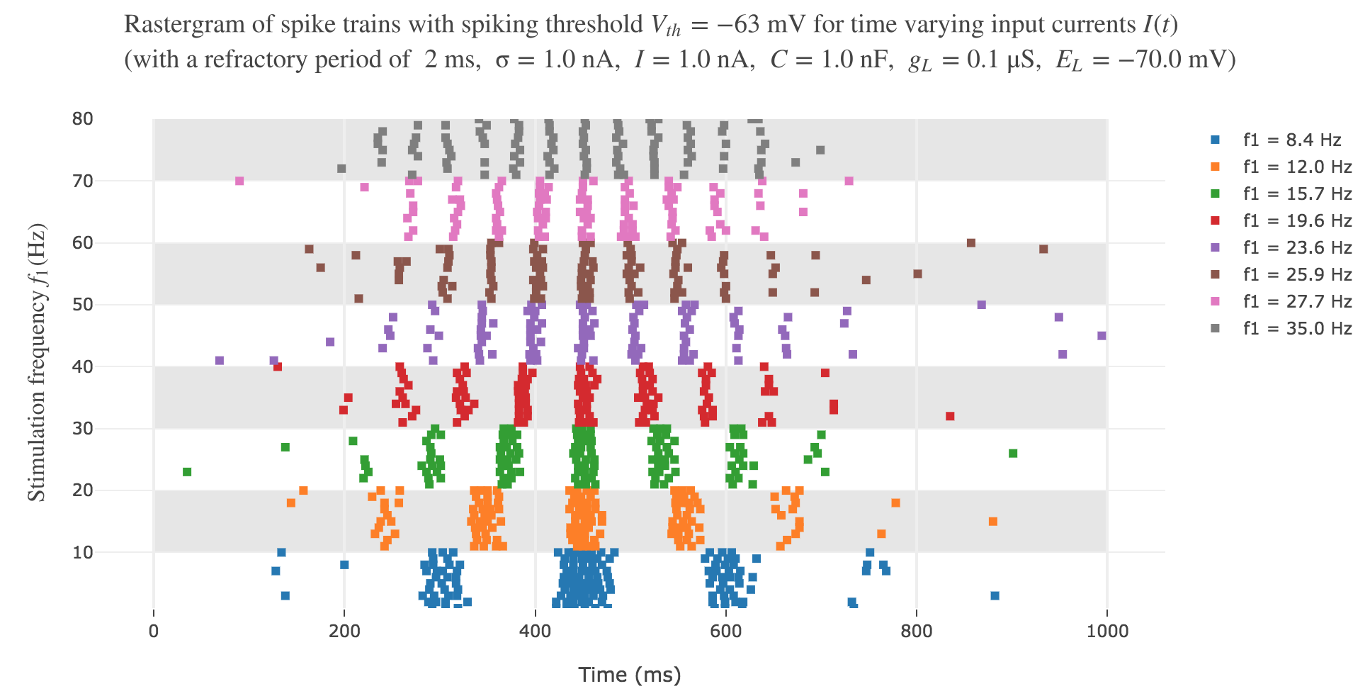
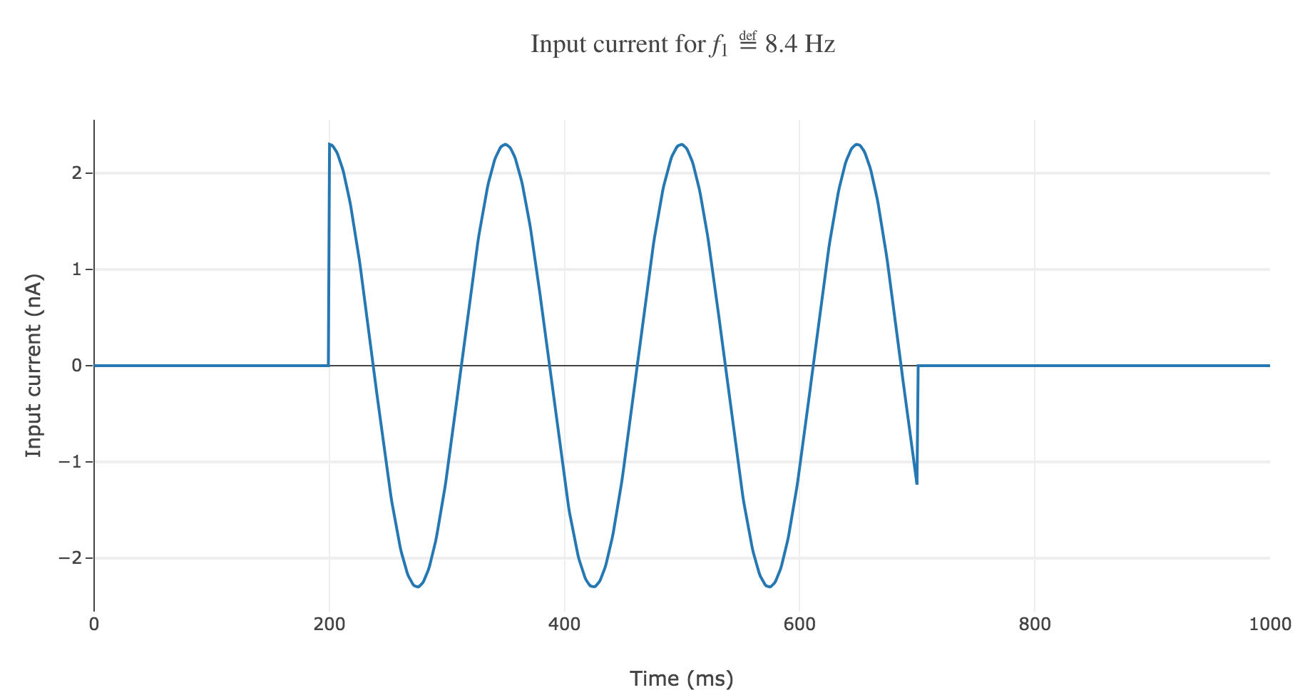
Another solution would be to go for a Heaviside envelope: the current is purely sinusoidal within the simulation period, it is equal to zero everywhere else.

The resulting time-varying input current

\[I(t) \propto \begin{cases} \cos(f_1 (t-200)/200) \text{ if } t∈[200, 700] \text{ ms} \\ 0 \text{ else} \end{cases}\]

could look like this:

Figure - Sinusoidal input current with a Heaviside envelope

The resulting rastergram:

Figure h.4. - Rastergram of artifical spike trains induced by a sinusoidal input current modulated by a Heaviside envelope, for various vibration frequencies

resembles way more to the experimental one!

However, the average spike count/firing rate as a function of the vibration frequency is not satisfying: it is somewhat anti-linear with respect to the vibration frequency!

Figure h.5. - Average spike count as a function of the vibration frequency with standard deviation errorbars

Figure h.6. - Average firing rate as a function of the vibration frequency with standard error of the mean $SEM = σ/ \sqrt{N}$ errorbars

This can be explained by the fact that even though the frequency of spikes increases with the vibration frequency $f_1$, the width of the “spikes fired in a row” is decreasing (since the sinusoidal current curve is becoming thinner and thinner, the current reaches high values during a shorter and shorter time as the frequency increases). To overcome that, we would have to ensure that the width of the current waves remains the same irrespective of the frequency: this can be achieved with square waves.

If the model somehow described what happens in reality, it would mean that the current injected though the membrane of the monkey’s primary somatosensory cortex neuron when a stimulus vibrates at a frequency $f_1$ on its fingertip is:

• null outside the simulation period
• sinusoidal within the simulation period

leading to a voltage accross the membrane reaching the threshold voltage periodically (the higher the vibration frequency, the smaller the period), which in turn induces an average firing rate depending linearly on $f_1$.