TP2: Optical flow

Read, understand, complete and run the following notebook. You must return the completed notebook, including your answers and illustrations (you may need to add cells to write your code or comments).

Return your work by e-mail using a single file (ipynb or zip) with the format 'introvis17_tp2_yourname.ipynb'

The first part implements two basic optical flow algorithm, minimizing pixel differences and patch correlation in a window. The second part implements a step of the Lukas Kanade algorithm.

0. Preliminaries

a) Re-use imports and meaningful functions (grayscale image loading and croping) from the first TP.

# /!\: I will resort to PYTHON3
import numpy as np 
import matplotlib.pyplot as plt 
%matplotlib inline 
import scipy.ndimage as ndimage
plt.rcParams['image.cmap'] = 'gray'

# Markdown
from IPython.display import display, Markdown

# Interact widget
from __future__ import print_function
from ipywidgets import interact, interactive, fixed, interact_manual
import ipywidgets as widgets

def load_image_v0(name,crop_window=-1): 
    I=plt.imread(name)
    if crop_window!=-1:
        I=I[crop_window[0]:crop_window[1],crop_window[2]:crop_window[3]] # slices the image according to crop_window
    I=I.astype('float')/255
    return I

def load_image(name,crop_window=-1): 
    I = load_image_v0(name, crop_window)
    
    # if the input is already grayscale,
    # i.e. if it's a 2D array, just return it
    if I.ndim == 2:
        return I
    else: 
        # it's a color image (3D array: there's an additional dimension for the RGB coordinates) 
        # The following dot product is a weighted sum over the RGB coordinates (last axis) of I, 
        #  whose weights are the values of [0.2989, 0.5870, 0.1140], which is what we want
        # (cf https://docs.scipy.org/doc/numpy/reference/generated/numpy.dot.html)
        return np.dot(I, np.array([0.2989, 0.5870, 0.1140]))

plt.imshow(plt.imread('traction1.tif'))
plt.show()
plt.imshow(plt.imread('road1.png'))

<matplotlib.image.AxesImage at 0x10dea7320>

b) Download the two following image pairs: traction 1 and 2; road 1 and 2.

The images (especially traction) are big, for most of the TP, it will be convenient to work with smaller crops from these images (both for speed and visualization). Check you can load and display them. Estimate the scale of the displacement in both pairs.

crop_window1 = [1450, 1550, 500, 700]
crop_window2 = [250, 350, 250, 450]

I_traction1, I_traction2 = load_image('traction1.tif', crop_window=crop_window1), load_image('traction2.tif', crop_window=crop_window1)
I_road1, I_road2 = load_image('road1.png', crop_window=crop_window2), load_image('road2.png', crop_window=crop_window2)

Images = [[I_traction1, I_traction2], [I_road1, I_road2]]
labels = ["Traction", "Road"] 

for imgs, label in zip(Images, labels):

    display(Markdown("#### {}".format(label)))
    fig = plt.figure(figsize = (15., 15.))
    
    for index, img in enumerate(imgs):
        fig.add_subplot(1, 3, index+1).set_title("{} {}".format(label, index+1))
        plt.imshow(img)
        plt.axis('off')

    fig.add_subplot(1, 3, 3).set_title("Difference (2 - 1)")
    plt.imshow(imgs[1] - imgs[0])
    plt.axis('off')

    plt.show()
    display(Markdown("\n \n_______"))

Traction

---

Road

---

According the difference images, it appears that:

1. For the traction images: the displacement is an overall top-to-bottom translation of size $≃ 3$ pixels

2. For the road images: the displacement of

   • the left car is right-to-left translation of size $≃ 2$ pixels
   • the right car is an overall left-to-right translation of size $≃ 5$ pixels

c) The following function allows to display a flow field as arrows on an image.

• I1 will be the image in the background (typically the first image of the pair on which the flow is computed)
• flow will be a pair of images corresponding to the horizontal and vertical displacements
• delta defines the postions at which flow is defined (on a grid, starting in delta+1 and with interval 2*delta+1 between each value: it's convenient when working with patches).
• The 'scale' parameters is such that a flow of size f is represented by an arrow of size f/scale.

This function will be used later, but you should understand and can test it now.

from matplotlib.pyplot import cm
def visualize_flow(I1,flow,delta, scale=0.5):
    H, W = I1.shape
    flow_i, flow_j = flow
    plt.figure(figsize = (10., 10.))
    plt.imshow(I1)
    Y, X = np.mgrid[delta:H-delta:2*delta+1, delta:W-delta:2*delta+1]
    plt.quiver(X, Y,     # position where the flow is computed
               flow_j, flow_i,        # flow
               np.sqrt(flow_i**2 + flow_i**2),      # colour the arrows based on this array
               cmap=cm.jet,     # colour map
               headlength=7, # length of the arrows head
               angles='xy', scale_units='xy', 
               scale=scale)  # scale of the arrows: a flow of 1 pixel is visualized by an arrow of 1/scale pixels

1. First coarse optical flow Algorithms

This part aim at implementing the first algorithms we have seen in the lecture to compute the best correspondence between images using local search in a small window and comparing pixel values (1.1) or image patches (1.2)

1.1. Minimizing pixel errors

The different methods will need parameters. For conveniency, we all store them in a single dictionnary structure named params that we will contain all the parameters and be given as argument to the different functions. For this first method, we have a single parameter, describing how far we will look for a correponding pixel.

params={}

# size of the window in which we search for the optimal. 
# The total size of the window in which we look for a correspondence is (2*params['search_window_half_size']+1)^2
params['search_window_half_size'] = 10 # you will need to adjust this value

Read and understand the following code

def compute_pixel_flow(I1, I2, params):
    d = params['search_window_half_size']
    # Width, Height
    W, H = I1.shape
    
    # Initializing flow
    flow_i, flow_j = np.zeros(I1.shape), np.zeros(I1.shape)
    
    for image_i in range(0,W):
        for image_j in range(0,H):
            # Fix a reference pixel
            ref = I1[image_i,image_j]
            
            # Initialize minimum value of absolute difference with the reference pixel 
            min_value = np.abs(ref-I2[image_i,image_j])
            
            for di in range(-d,d+1):
                # if outside the range of the array: pass
                if image_i+di<0 or image_i+di>W-1:
                    continue
                for dj in range(-d,d+1):
                    # if outside the range of the array: pass
                    if image_j+dj<0 or image_j+dj>H-1:
                        continue
                    
                    # Compare the current absolute difference with the reference pixel
                    # with the current minimum -> update it if smaller
                    candidate_value = np.abs(ref-I2[image_i+di,image_j+dj])
                    if candidate_value < min_value:
                        min_value = candidate_value
                        
                        # the current minimum absolute difference is reached for the
                        # current pixel, corresponding to a relative displacement
                        # of (di, dj) with respect to the reference pixel 
                        # -> update the flow accordingly
                        flow_i[image_i,image_j], flow_j[image_i,image_j] = di, dj

    return flow_i, flow_j

a) Describe in a few sentences and simple words what this code is doing

This algorithm computes the flow at position [i, j] for each reference pixel [i, j] in the image by

• computing at which surrounding (i.e. in a window of size $d×d$) pixel [i+di, j+dj] the absolute difference with the reference pixel is reached ($-d ≤ di, dj ≤ d$)
• setting the flow at position [i,j] to [di, dj] (the displacement vector is [i+di, j+dj] - [i,j])

b) Try your code on the two image pairs. Visualize each of the flow (horizontal and vertical) as grayscale images and print some values. Try with different parameters and comment.

Warning: this code is slow! You can take small (e.g. 100×100) patches from the images to test it in a reasonnable time.

Note: whatever you do, the results won't look very good, but you should still be able to make a few observations.

labels_flow = ["flow_i", "flow_j"] 

def show_flow(win_half_size, I, label):
    
    params['search_window_half_size'] = win_half_size
    flow = compute_pixel_flow(I[0], I[1], params)
    fig = plt.figure(figsize = (15., 15.))
    
    for index, img in enumerate(flow):
        fig.add_subplot(1, 3, index+1).set_title("{} {}".format(label, labels_flow[index]))
        plt.imshow(img)
        plt.axis('off')
    plt.show()
    display(Markdown("- **Shape of the images:** `{}` \n"\
                 "- **Search window half size**: `{}` \n"\
                 "> Mean displacement (in pixels): `{}` \n"\
      .format(I[0].shape, win_half_size, np.mean(np.sqrt(flow[0]**2+ flow[1]**2)))))

---

Preview image (of the cell below)

---

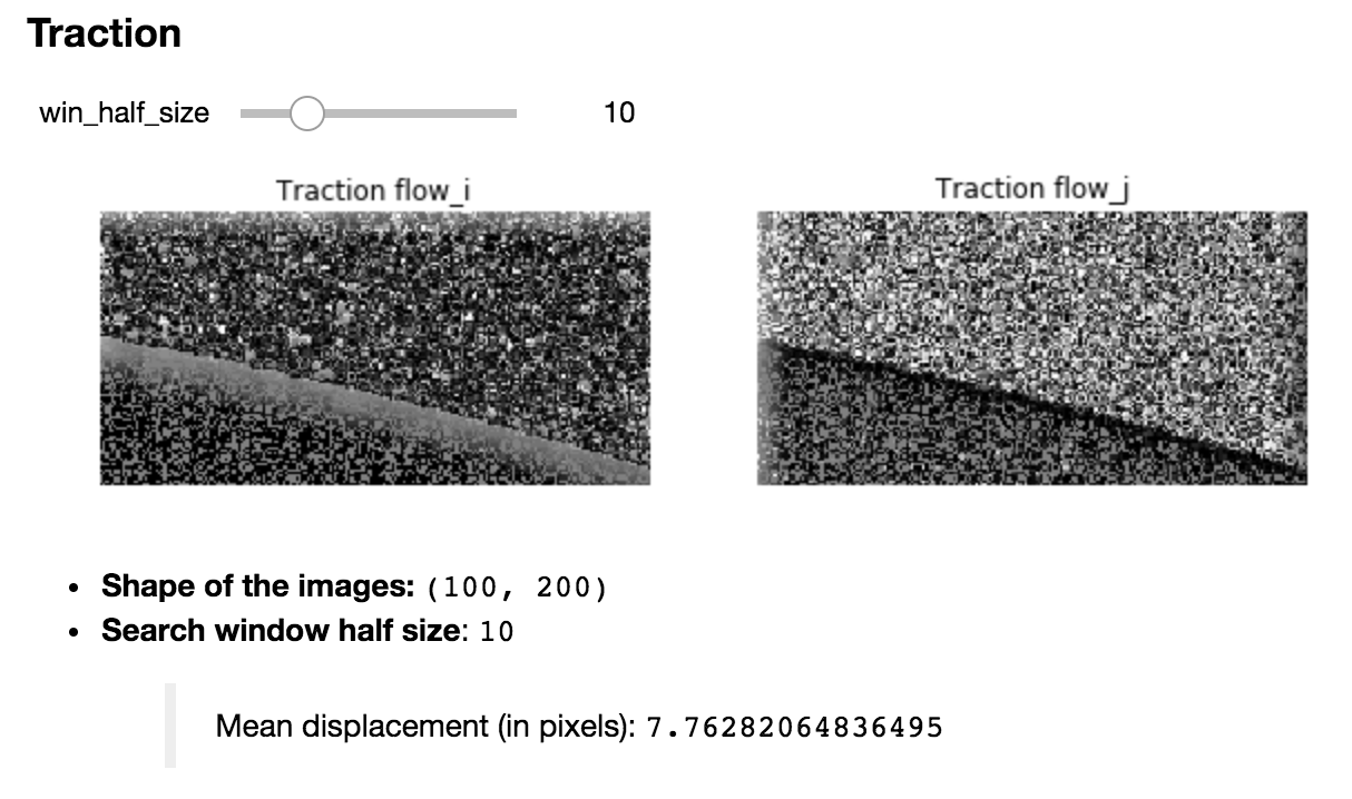
label = "Traction"
Imgs = [I_traction1, I_traction2]

display(Markdown("### {}".format(label)))

interact(show_flow, win_half_size=widgets.IntSlider(min=1,max=40,step=1,value=10),\
         label=fixed(label), I=fixed(Imgs));

Traction

---

Preview image (of the cell below)

---

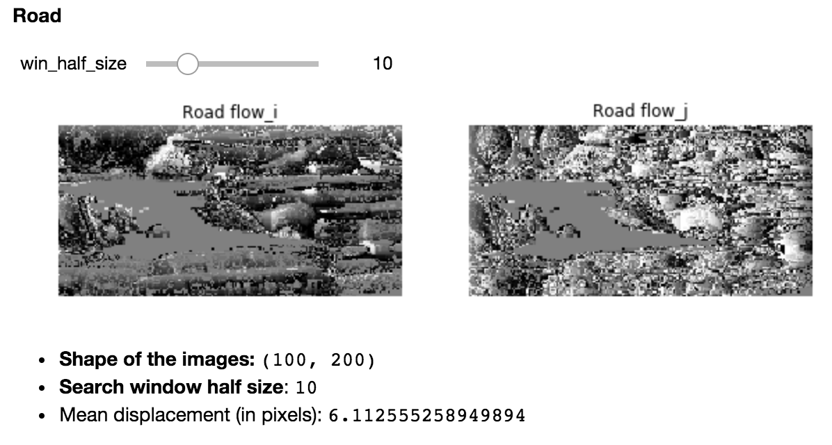
label = "Road"
Imgs = [I_road1, I_road2]

display(Markdown("### {}".format(label)))

interact(show_flow, win_half_size=widgets.IntSlider(min=1,max=40,step=1,value=10),\
         label=fixed(label), I=fixed(Imgs));

Road

Comments

1. By increasing the window half size, one increases the mean displacement (as expected).
2. For the traction images: the bright values of the flow along j point at the fact that the image is globally translated vertically

3. For the road images:

   • one distinguishes the outline of the left car (the uniformally gray area), indicating that the movement of the left car is uniform
   • whereas the stripes near the location of the right car hint at an overall movement of the latter towards the right.

1.2. Maximizing correlations

To obtain better results, we will maximize correlation instead of simply minimizing the distance between the image value for each pixel. We now have two parameters: how far we look for a correspondence (similar to 1.1) and the size of the patches we compare.

params={}

# size of the patches to compare
# similar to before, the size of the patches is (2*params['patch_size']+1)^2
params['patch_half_size']=3 # you will need to adjust this value

# size of the window in which we search for the optimal
params['search_window_half_size']=10 # you will need to adjust this value

a) Write a function patch_similarity which returns the zero normalized cross-correlations between two input patches (P1 and P2)

def patch_similarity(P1, P2):
    # Compute ZNCC as defined here:
    # http://imagine.enpc.fr/~aubrym/lectures/introvis17/lecture_4.pdf (slide 56)
    mu_1 = np.sum(P1)
    mu_2 = np.sum(P2)
    sigma_1 = np.sqrt(np.sum((P1 - mu_1)**2))
    sigma_2 = np.sqrt(np.sum((P2 - mu_2)**2))
    return np.sum((P1 - mu_1)/sigma_1 * (P2 - mu_2)/sigma_2)

b) Complete the function compute_zncc_flow to compute the optimal displacement for each patch in an image. For efficiency, we don't consider overlaping patches.

def compute_zncc_flow(I1,I2,params):
    d_corr=params['patch_half_size']
    d_search=params['search_window_half_size']
    delta=2*d_corr+1
    W=I1.shape[0]
    H=I1.shape[1]
    flow_i=np.zeros([len(list(range(d_corr,W-d_corr,delta))),len(list(range(d_corr,H-d_corr,delta)))])
    flow_j=np.zeros([len(list(range(d_corr,W-d_corr,delta))),len(list(range(d_corr,H-d_corr,delta)))])
    
    # for all the reference center pixels (at the center of a patch)
    for image_i in range(d_corr,W-d_corr,delta):
        for image_j in range(d_corr,H-d_corr,delta):
            
            # compute the reference patch associated with it
            ref=I1[image_i-d_corr:image_i+d_corr+1,image_j-d_corr:image_j+d_corr+1]
            
            # initialize the maximum patch similarity value
            # with the one for the current patch
            max_value=patch_similarity(ref,I2[image_i-d_corr:image_i+d_corr+1,image_j-d_corr:image_j+d_corr+1])
            
            # for all displacement (di, dj) in a surrounding window of size d_search x d_search
            for di in range(-d_search,d_search+1):
                if image_i+di-d_corr<0 or image_i+di+d_corr>W-1:
                    continue
                for dj in range(-d_search,d_search+1):
                    if image_j+dj-d_corr<0 or image_j+dj+d_corr>H-1:
                        continue
                    
                    # compute the patch similarity between the patch of the current surrounding pixel
                    # and the reference patch
                    val=patch_similarity(ref,I2[image_i+di-d_corr:image_i+di+d_corr+1,image_j+dj-d_corr:image_j+dj+d_corr+1])
                    
                    # update the flow estimate if this patch similarity is the maximal one so far
                    if val > max_value:
                        max_value = val
                        
                        # set the flow corresponding to the current position
                        # to the current displacement (di, dj)
                        ind_i = int((image_i-d_corr)/delta)
                        ind_j = int((image_j-d_corr)/delta)
                        flow_i[ind_i,ind_j] = di
                        flow_j[ind_i,ind_j] = dj
    return flow_i, flow_j

c) Compute the flows using your function between the two pairs of images. As before, visualize them as images and print the values. Comment on the results and choice of parameters.

labels_flow = ["flow_i", "flow_j"] 

def show_flow_zncc(win_half_size, patch_half_size, I, label):
    
    params['search_window_half_size'] = win_half_size
    params['patch_half_size'] = patch_half_size

    flow = compute_zncc_flow(I[0], I[1], params)
    fig = plt.figure(figsize = (15., 15.))
    
    for index, img in enumerate(flow):
        fig.add_subplot(1, 3, index+1).set_title("{} {}".format(label, labels_flow[index]))
        plt.imshow(img)
        plt.axis('off')
    plt.show()
    display(Markdown("- **Shape of the images:** `{}` \n"\
                 "- **Search window half size**: `{}` \n"\
                 "- **Patch half size**: `{}` \n"\
                 "> Mean displacement (in pixels): `{}` \n"\
      .format(I[0].shape, win_half_size, patch_half_size, np.mean(np.sqrt(flow[0]**2+ flow[1]**2)))))

---

Preview image (of the cell below)

---

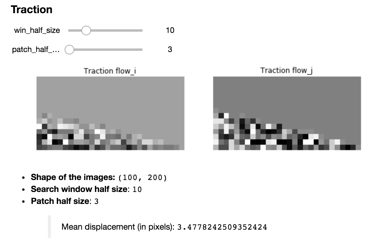
label = "Traction"
Imgs = [I_traction1, I_traction2]

display(Markdown("### {}".format(label)))

interact(show_flow_zncc, win_half_size=widgets.IntSlider(min=1,max=40,step=1,value=10),\
         patch_half_size=widgets.IntSlider(min=3,max=30,step=1,value=3),\
         I=fixed(Imgs), label=fixed(label),\
         scale=widgets.FloatSlider(min=0.1,max=1,step=0.05,value=1));

Traction

---

Preview image (of the cell below)

---

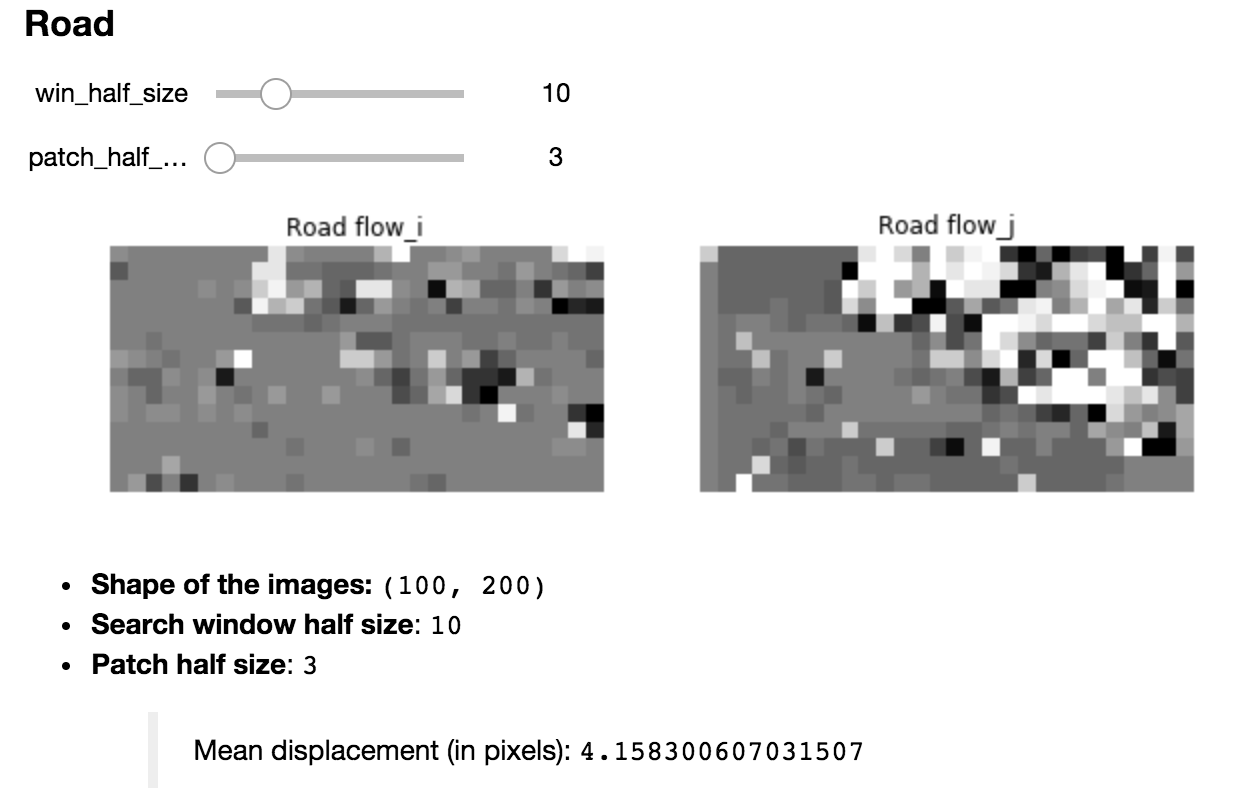
label = "Road"
Imgs = [I_road1, I_road2]

display(Markdown("### {}".format(label)))

interact(show_flow_zncc, win_half_size=widgets.IntSlider(min=1,max=40,step=1,value=10),\
         patch_half_size=widgets.IntSlider(min=3,max=30,step=1,value=3),\
         I=fixed(Imgs), label=fixed(label),\
         scale=widgets.FloatSlider(min=0.1,max=1,step=0.05,value=1));

Road

Comments

1. By increasing the window half size, one increases the mean displacement, but not as much as for compute_pixel_flow (as expected: the zncc approach is less sensitive to noisy values)
2. By increasing the patch half size, one decreases the mean displacement: as the minimum zncc is less likely to be reached at another surrounding pixel, since patches are bigger.

3. For the traction images: the flow indicates

   • a uniform displacement (grey area) outside the black area in the original image
   • and scattered (ranging from almost nothing (black regions) to significant movement (white regions)) displacement around the black area in the original image.
4. For the road images: the flow points at a displacement globally located on the right (corresponding to the right car)

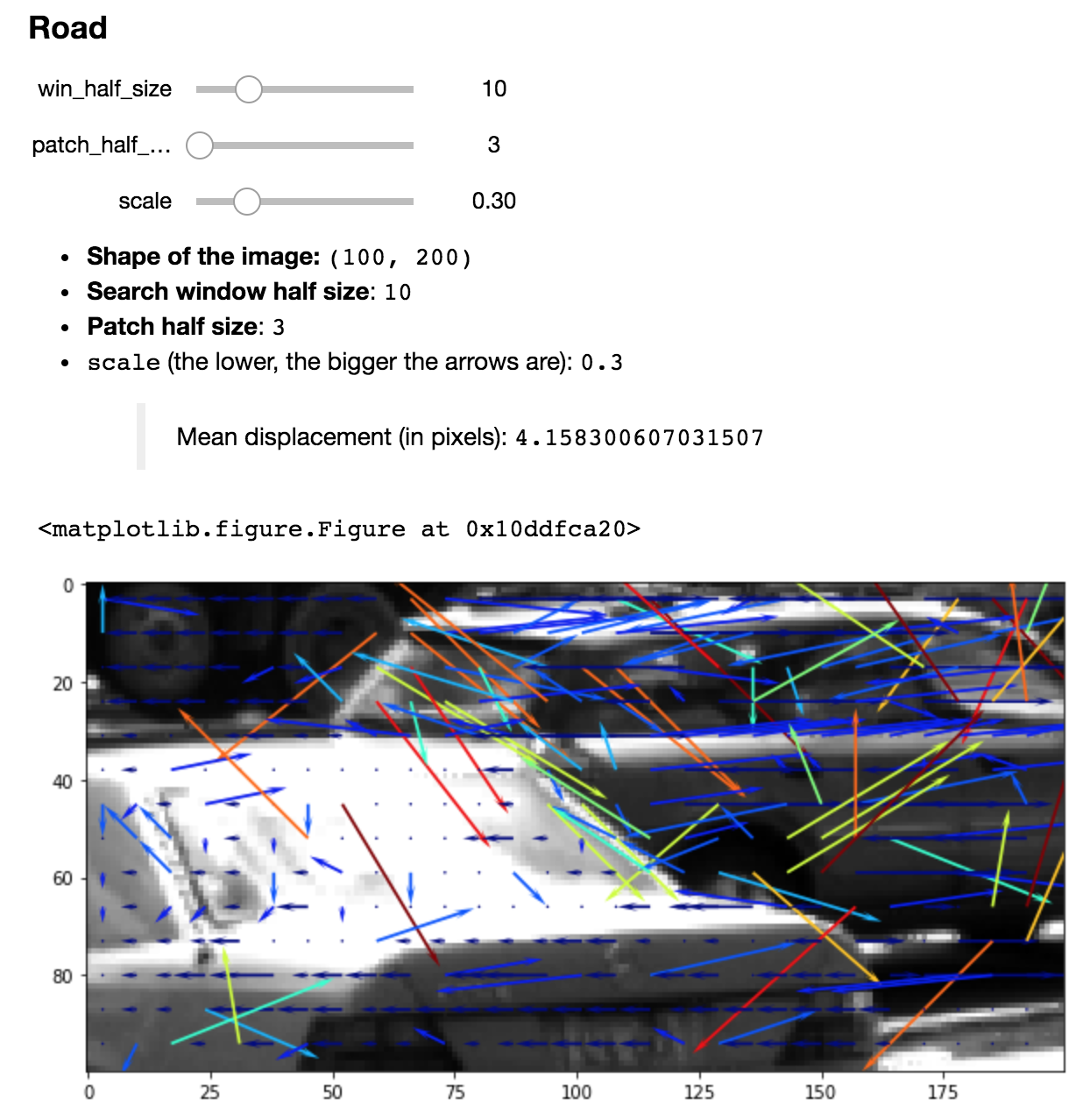
d) Use the visualize_flow function defined in the preliminaries to visualize the flow as an arrow field. What should be the value of the delta parameter? What should be the scale parameter for each image pair?

Note: the flow you obtain with this algorithm should be meaningful!

labels_flow = ["flow_i", "flow_j"] 

def show_flow_zncc2(win_half_size, patch_half_size, I, scale=1):
    
    params['search_window_half_size'] = win_half_size
    params['patch_half_size'] = patch_half_size
    flow = compute_zncc_flow(I[0], I[1], params)
    fig = plt.figure(figsize = (15., 15.))
    
    visualize_flow(I[0], flow, patch_half_size, scale=scale)
    
    display(Markdown("- **Shape of the image:** `{}` \n"\
                 "- **Search window half size**: `{}` \n"\
                 "- **Patch half size**: `{}` \n"\
                 "- `scale` (the lower it is, the bigger the arrows are): `{}` \n"\
                 "> Mean displacement (in pixels): `{}` \n"\
      .format(I[0].shape, win_half_size, patch_half_size, scale,\
              np.mean(np.sqrt(flow[0]**2+ flow[1]**2)))))

---

Preview image (of the cell below)

---

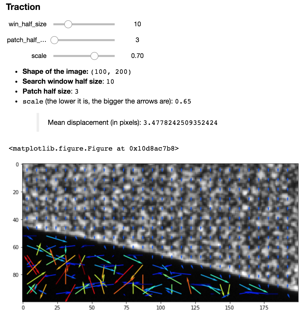
label = "Traction"
Imgs = [I_traction1, I_traction2]

display(Markdown("### {}".format(label)))

interact(show_flow_zncc2, win_half_size=widgets.IntSlider(min=1,max=40,step=1,value=10),\
         patch_half_size=widgets.IntSlider(min=3,max=30,step=1,value=3),\
         I=fixed(Imgs), scale=widgets.FloatSlider(min=0.1,max=1,step=0.05,value=0.7));

Traction

---

Preview image (of the cell below)

---

label = "Road"
Imgs = [I_road1, I_road2]

display(Markdown("### {}".format(label)))

interact(show_flow_zncc2, win_half_size=widgets.IntSlider(min=1,max=40,step=1,value=10),\
         patch_half_size=widgets.IntSlider(min=3,max=30,step=1,value=3),\
         I=fixed(Imgs), scale=widgets.FloatSlider(min=0.1,max=1,step=0.05,value=0.3));

Road

Comments

• the delta parameter should be equal to params['patch_half_size']

• the scale parameter should be:

  • around 0.7 for the traction images (to distinguish the top-to-bottom translation)
  • around 0.3 for the road images (to see the movements of the two cars going forward)

3. Lukas Kanade

We will implement a single step from the algorithm (no iteration, phi=Id)

a) Complete the following function (note: we only compute the flow on a grid, of which size is defined by params['patch_half_size']).

def lucas_kanade_step(I1,I2,params):
    d = params['patch_half_size']
    delta=2*d+1
    W=I1.shape[0]-2
    H=I1.shape[1]-2
    flow_i=np.zeros([len(list(range(d,W-d,delta))),len(list(range(d,H-d,delta)))])
    flow_j=np.zeros([len(list(range(d,W-d,delta))),len(list(range(d,H-d,delta)))])
    
    # compute the image derivative in x and y, using a small gaussian blur, as well as the difference between the two images
    I1 = ndimage.gaussian_filter(I1, sigma=params['sigma']) 
    I2 = ndimage.gaussian_filter(I2, sigma=params['sigma'])
    I_x = np.array([[I1[i,j]-I1[i-1,j] for j in range(1, H+1)] for i in range(1, W+1)])
    I_y = np.array([[I1[i,j]-I1[i,j-1] for j in range(1, H+1)] for i in range(1, W+1)])
        
    I_t = I1[1:-1, 1:-1] - I2[1:-1, 1:-1]
    
    # using the derivative you just compute the products that will be used in the dispacement computations
    I_xx=I_x*I_x
    I_xy=I_x*I_y
    I_yy=I_y*I_y
    I_xt=I_x*I_t
    I_yt=I_y*I_t
    
    
    # we will only compute the flow for disjoint patches
    for image_i in range(d,W-d,delta):
        for image_j in range(d,H-d,delta):
            ref_i=image_i-d
            ref_j=image_j-d
            
            # compute the terms of A, tA, tAb and det(tAA)
            sum_I_xx = np.sum(I_xx[ref_i:ref_i+delta,ref_j:ref_j+delta])
            sum_I_xy = np.sum(I_xy[ref_i:ref_i+delta,ref_j:ref_j+delta])
            sum_I_yy = np.sum(I_yy[ref_i:ref_i+delta,ref_j:ref_j+delta])
            sum_I_xt = np.sum(I_xt[ref_i:ref_i+delta,ref_j:ref_j+delta])
            sum_I_yt = np.sum(I_yt[ref_i:ref_i+delta,ref_j:ref_j+delta])
            
            det=sum_I_xx*sum_I_yy-sum_I_xy*sum_I_xy
            
            # complete to compute the flow. You  need to test whether det is 0 or not
            assert det != 0
            ind_i, ind_j = int(ref_i/delta), int(ref_j/delta)
            flow_i[ind_i, ind_j], flow_j[ind_i, ind_j] = np.linalg.solve(np.array([[sum_I_xx, sum_I_xy], [sum_I_xy, sum_I_yy]]),\
                                                                         np.array([sum_I_xt, sum_I_yt]))

            
    return flow_i, flow_j

b) Test your algorithm on the traction image and comment the results.

params['patch_half_size'] = 6
params['search_window_half_size'] = 10 
params['sigma'] = 3

flow = lucas_kanade_step(I_traction1, I_traction2, params)
visualize_flow(I_traction1, flow, 6.05, scale=0.2)

params['patch_half_size'] = 100

I1=load_image('traction1.tif',[0,2000,0,2000])
I2=load_image('traction2.tif',[0,2000,0,2000])

flow = lucas_kanade_step(I1,I2,params)

visualize_flow(I1,flow, params['patch_half_size'], scale=0.01)

Comments

One clearly sees the top-to-bottom translation, down until the black area.

c) Here is a basic algorithm to iterate the step function. Comment it (the function of each block of code should be explained, similar to the step function above).

# note: a coarse to fine approach is necessary for good results. To keep things simple I simply blur the image 
# with Gaussians of decreasing size. I set it up so that the maximum displacement is of the order of 2^(n_iter/4)
# Something better is clearly possible. Also, I kept the patch approach you mentionned was used in mechanics. 
# I think working densely would be better
def lucas_kanade_full(I1,I2,params):
    d=params['patch_half_size']
    delta=2*d+1
    N0=int(I1.shape[0]/delta)*delta
    N1=int(I1.shape[1]/delta)*delta
    
    # Preparing the meshgrid
    # Exactly equivalent to doing:
    # interp_coo_i_ref, interp_coo_j_ref = np.mgrid[0:N0, 0:N1]
    # interp_coo_ref = np.concatenate([[X],[Y]], axis=0)
    #
    # interp_coo_i, interp_coo_j = np.mgrid[0:N0, 0:N1]
    # interp_coo_i, interp_coo_j = (interp_coo_i - d)/delta, (interp_coo_j - d)/delta
    # interp_coo = np.concatenate([[X],[Y]], axis=0)
    
    interp_coo_i_ref=np.repeat(
        np.reshape((np.array(range(0, N0))).astype('float'),[1,-1,1]), 
        N1,axis=2)
    interp_coo_j_ref=np.repeat(
        np.reshape((np.array(range(0, N1))).astype('float'),[1,1,-1]),
        N0,axis=1)
    interp_coo_ref=np.concatenate([interp_coo_i_ref,interp_coo_j_ref], axis=0)
    
    interp_coo_i=np.repeat(
        np.reshape((np.array(range(0, N0)).astype('float')-d)/delta,[1,-1,1]), 
        N1,axis=2)
    interp_coo_j=np.repeat(
        np.reshape((np.array(range(0, N1)).astype('float')-d)/delta,[1,1,-1]),
        N0,axis=1)
    interp_coo=np.concatenate([interp_coo_i,interp_coo_j], axis=0)
    
    # Cropping the images to avoid border issues
    I1_t=I1[:N0,:N1]
    I2_t=I2[:N0,:N1]
    
    # Initialization
    print('initial error = ' + str(np.mean((I1_t-I2_t)**2)))
    flow_i_tot=[]
    flow_j_tot=[]
    full_coo=[]
    N=params['n_iter']
    
    for t in range(0,N):
        # New gaussian standard deviation (whose size decreases with respect to t: coarse-to-fine approach)
        params['sigma']=params['sigma0']/np.sqrt(float(t+1))
        print('sigma ='+str(params['sigma']))
        
        # Lukas Kanade step with this smaller (thus finer) gaussian standard deviation
        flow_i,flow_j=lucas_kanade_step(I1_t,I2_t,params)
        
        # Adding the computed flow at this step to the current flow, 
        # to refine the estimation
        if t==0:
            flow_i_tot=params['step_size']*flow_i
            flow_j_tot=params['step_size']*flow_j
        else:
            flow_i_tot+=params['step_size']*flow_i
            flow_j_tot+=params['step_size']*flow_j
        
        # To get the full flow, one fills in the gaps by interpolating
        # the flow values at positions given by the meshgrid interp_coo
        flow_i_full=ndimage.interpolation.map_coordinates(flow_i_tot,interp_coo,mode='nearest')
        flow_j_full=ndimage.interpolation.map_coordinates(flow_j_tot,interp_coo,mode='nearest')
        
        # Concatenating the "full flow" obtained along i and j into one full_coo array
        full_coo=np.concatenate(
            [np.reshape(flow_i_full,[1,flow_i_full.shape[0],flow_i_full.shape[1]]),
            np.reshape(flow_j_full,[1,flow_j_full.shape[0],flow_j_full.shape[1]])],
            axis=0
        )
        
        # Updating I2_t, by interpolating I2 values at positions given by interp_coo_ref+full_coo :
        #   the reference interpolating coordinates (the inital meshgrid)
        # + the full flow coordinates currently computed
        # which amounts to retrieving the positions of the (currently estimated) matching pixels
        # in I2 (that is, the pixels obtained after applying the (currently estimated) displacement)
        I2_t= ndimage.interpolation.map_coordinates(I2,interp_coo_ref+full_coo,mode='nearest')    
        
        print('error = ' +str(np.mean((I1_t-I2_t)**2)))
    return full_coo, I2_t, I1_t, flow_i_full, flow_j_full 

d) Try it on the traction images (parameters given below) and visualize it using the visualize_flow function (the function outputs a dense flow, you will need to extract a sparse flow from it).

params['n_iter']=5
params['step_size']=1

params['patch_half_size']=100
params['sigma0']=5

I1=load_image('traction1.tif',[0,2000,0,2000])
I2=load_image('traction2.tif',[0,2000,0,2000])

full_coo, I2_t, I1_t, flow_i_full, flow_j_full = lucas_kanade_full(I1, I2, params)

visualize_flow(I1_t, [flow_i_full[::200, ::200], flow_j_full[::200, ::200]], 85, scale=0.015)

initial error = 0.00976839115286
sigma =5.0
error = 4.48630265951e-05
sigma =3.53553390593
error = 4.38991424767e-05
sigma =2.88675134595
error = 4.38326100854e-05
sigma =2.5
error = 4.38069430699e-05
sigma =2.2360679775
error = 4.37953628805e-05

e) The results of the previous algo should be mainly a translation: what is its size in pixels? Remove the translation from the flow and visualize the remaining deformation.

display(Markdown("> **Size of the translation (in pixels):** `{}` \n"\
      .format(np.mean(np.sqrt(flow_i_full**2+ flow_j_full**2)))))

flow_i_without_trans, flow_j_without_trans = flow_i_full - np.mean(flow_i_full), flow_j_full - np.mean(flow_j_full)

visualize_flow(I1_t, [flow_i_without_trans[::200, ::200], flow_j_without_trans[::200, ::200]], 85, scale=0.00015)

Size of the translation (in pixels): 1.6581812598590944

display(Markdown("> **Size of the resulting deformation (in pixels):** `{}` \n"\
      .format(np.mean(np.sqrt(flow_i_without_trans**2+ flow_j_without_trans**2)))))

Size of the resulting deformation (in pixels): 0.01690070909459436