Dimensionality Reduction & Visualization of Representations
Younesse Kaddar
Studied articles: Visualizing MNIST, Visualizing Representations (C. Olah), Visualizing Data using t-SNE (L. Van der Maaten & G. Hinton) + Isomap & LLE
Introduction: Dimensionality reduction
I. MDS, Sammon’s mapping & Force-directed Graph Drawing
II. Principal component analysis (PCA)
III. Isomap
IV. Locally-Linear Embedding (LLE)
V. t-SNE & Meta-SNE
I. Introduction
Dimensionality Reduction
high-dimensional data$\qquad \rightsquigarrow \qquad \underbrace{\textit{lower-dimensional data}}_{\text{easier to visualize}}$
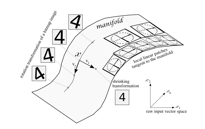
Manifold hypothesis: real-world high-dimensional data vectors lie in a lower-dimensional embedded manifold.
I.A - Multidimensional Scaling (MDS)
Goal: Preserve distances between points ⟹ conserve geometry
Gradient descent to minimize
I.B - Sammon’s mapping
The smaller the original distance between points is, the more preserved it is
Cost function to minimize:
I.C - Force-directed Graph Drawing
Build the graph where each point is connected to its $k$ nearest neighbors in original space, then:
Graph Physical analogy vertices repelling charged particles edges springs
As with electric potential energy and spring energy, minimize the potential energy function:
$\displaystyle \sum\limits_{x_i ≠ x_j \text{ data points}} \frac{1}{d^\ast(x_i, x_j)}$ $+$ $\displaystyle \sum\limits_{x_i, x_j \text{ data points}} \frac 1 2 \Big(d^\ast(x_i, x_j) - d(x_i, x_j)\Big)^2$
II. Principal component analysis (PCA)
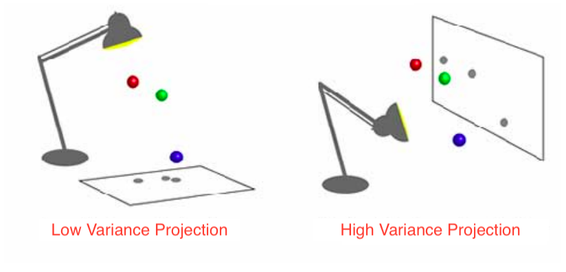
Goal: Find orthogonal axes onto which the variance of the data points under projection is maximal, i.e. find the best possible “angles” from which the data points are the most spread out.
III. Isomap
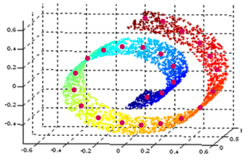
Goal: MDS but curvature of the data space taken into account
- ⟶ geodesic distance:
- length of paths on curved manifold surfaces are measured as if they were flat
IV. Locally-Linear Embedding (LLE)
Goal: Preserve the relationship between neighbors.
-
Find the weight matrix $(W_{i,j})_{i,j}$ - whose rows sum to $1$ - that minimizes
$$\sum\limits_{x_i \text{ data point}} \Big\vert \; x_i - \sum\limits_{x_j \text{ neighbor of } x_i} W_{i, j} x_j \;\Big\vert^2$$ -
Map each data point $x_i$ to a point $y_i$ in the vizualization, s.t. the $y_k$'s minimize
$$\sum\limits_{y_i \text{ data point}} \Big\vert \; y_i - \sum\limits_{y_j \text{ neighbor of } y_i} W_{i, j} y_j \;\Big\vert^2$$
t-Distributed Stochastic Neighbor Embedding (t-SNE)
Map points are:
- attracted to points that are near them in the data set
- repelled by points that are far from them in the data set
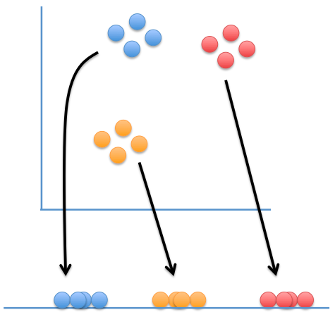
Image courtesy of statquest.org
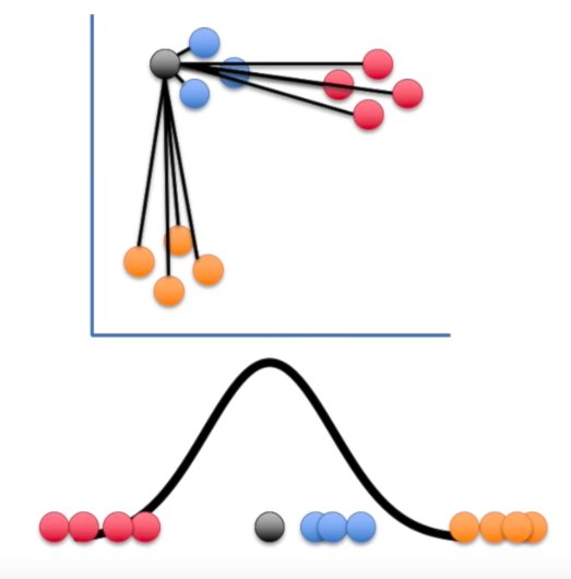
Step 1
probability that $x_i$ has $x_j$ as its neighbor if neighbors were chosen according to a Gaussian distribution centered at $x_i$
Step 2
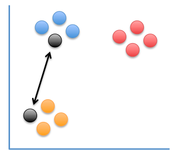
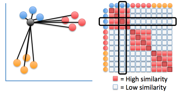
Step 3
-
$y_i$'s initialized at random
-
Similarities between visualization points:
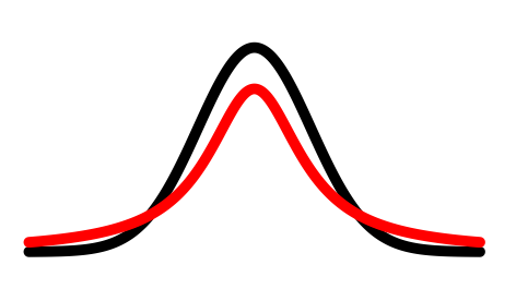
$$q_{i,j} ≝ \frac{(1+\vert\vert y_i-y_j\vert\vert^2)^{-1}}{\sum_{k\neq l}(1+\vert\vert y_i-y_l\vert\vert^2)^{-1}}$$⟶ computed with resort to a Student-$t$ distribution
Step 4
-
Minimize the Kullback–Leibler divergence: $C ≝ \sum_{i≠ j}p_{ij}\log {\frac {p_{i,j}}{q_{i,j}}}$, by modifying the $y_i$'s with gradient descent
-
Recompute the $q_{i,j}$'s at each step (until convergence is reached)
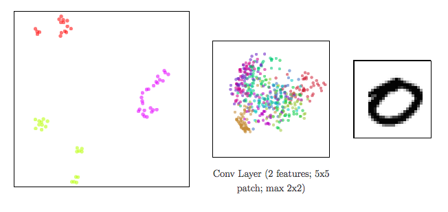
Dimensionality reduction to visualize high-dimensional representations
In a neural network:
- input data ⟶ shape changed from a layer to another: a representation is the reshaped data at a given layer.
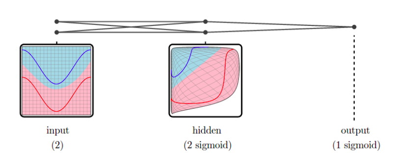
Since representations are high-dimensional ⟹ DR methods to visualize them
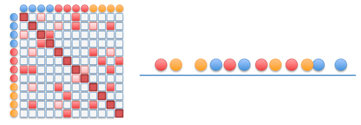
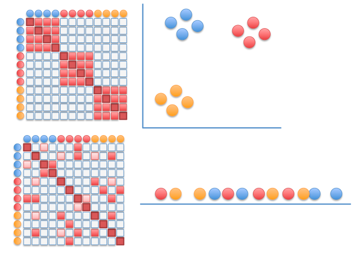
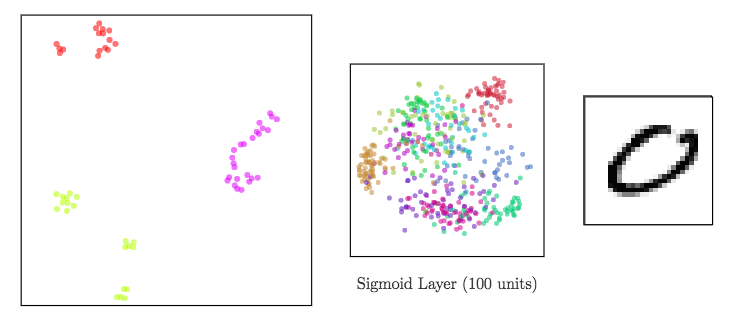
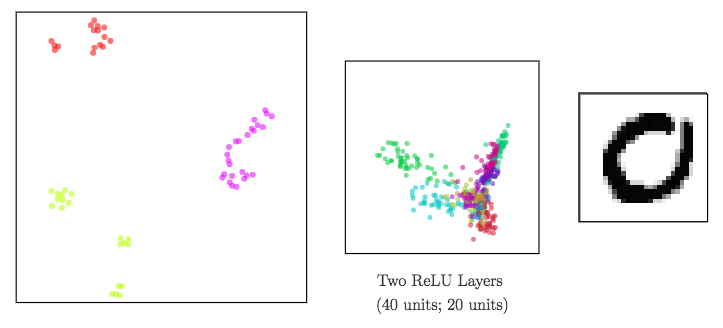
meta-SNE to visualize the space of representations
-
Build matrices of pairwise distances:
$$D_X ≝ \left(d_X(x_i, x_j)\right)_{i,j}$$⟹ vectorize representations -
Step up the ladder of abstraction: visualize vectorized representations with t-SNE
Regarding neural networks: meta-SNE enables us no longer to confine ourselves to comparing their outcome only, but also how they operate internally.
Sigmoid
ReLU
CNN
