Problem Set 2: Quantitative models of behavior
AT2 – Neuromodeling: Problem set #2 QUANTITATIVE MODELS OF BEHAVIOR
Younesse Kaddar
PROBLEM 1 - Rescorla-Wagner Model
Link of the iPython notebook for the code
Let us model a classical conditioning experiment with resort to the Rescorla-Wagner rule.
The experiment is as follows: at trial $i ∈ ℕ$:
- an animal may or may not be presented with a stimulus $u_i$ (e.g.: ringing a bell, clapping hands): $u_i = 1$ if the stimulus is present, $u_i = 0$ otherwise
- … which may or may not in turn be followed by a reward $r_i$ (e.g.: food): $r_i = 1$ if there is a reward, $r_i = 0$ otherwise
The animal is assumed to be willing to predict the correlation between the stimulus and the reward (e.g: by salivating in anticipation): i.e. to predict if it will get the reward based on the presence or absence of the stimulus. As such, the prediction of the animal is denoted by $v_i$ at trial $i$:
\[∀i, \; v_i ≝ w_i u_i\]where $w$ is a parameter learned and updated - trial after trial - by the animal, in accordance with the following Rescola-Wagner rule:
\[w_i → w_i + \underbrace{ε}_{\text{learning rate } << 1} \underbrace{(r_i − v_i)}_{≝ \, δ_i} u_i\]1. Introductory example
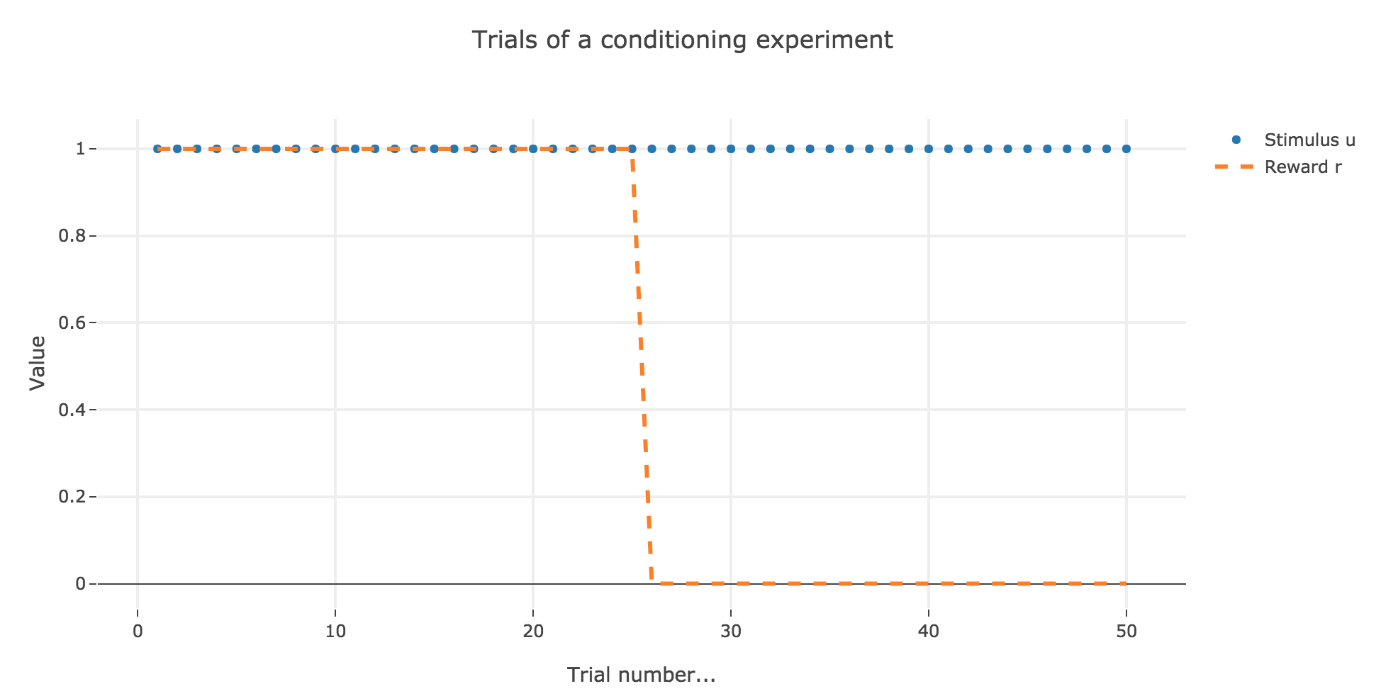
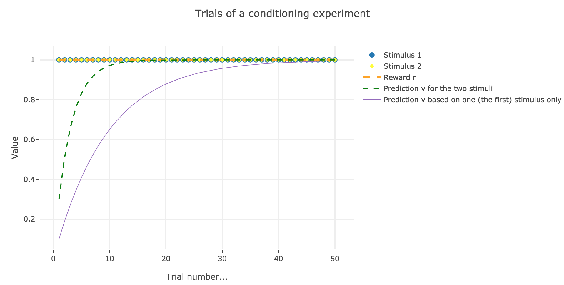
For instance, let us suppose that there are $50$ trials, and:
- during the first $25$ trials, both stimuli and reward are present ($u_i = r_i = 1$)
- during the last $25$ ones, only the stimulus is present ($u_i = 1, \, r_i = 0$)
as illustrated by the following figure:
In which case, according to the Rescola-Wagner rule, the animal prediction $v_i$ is as follows:
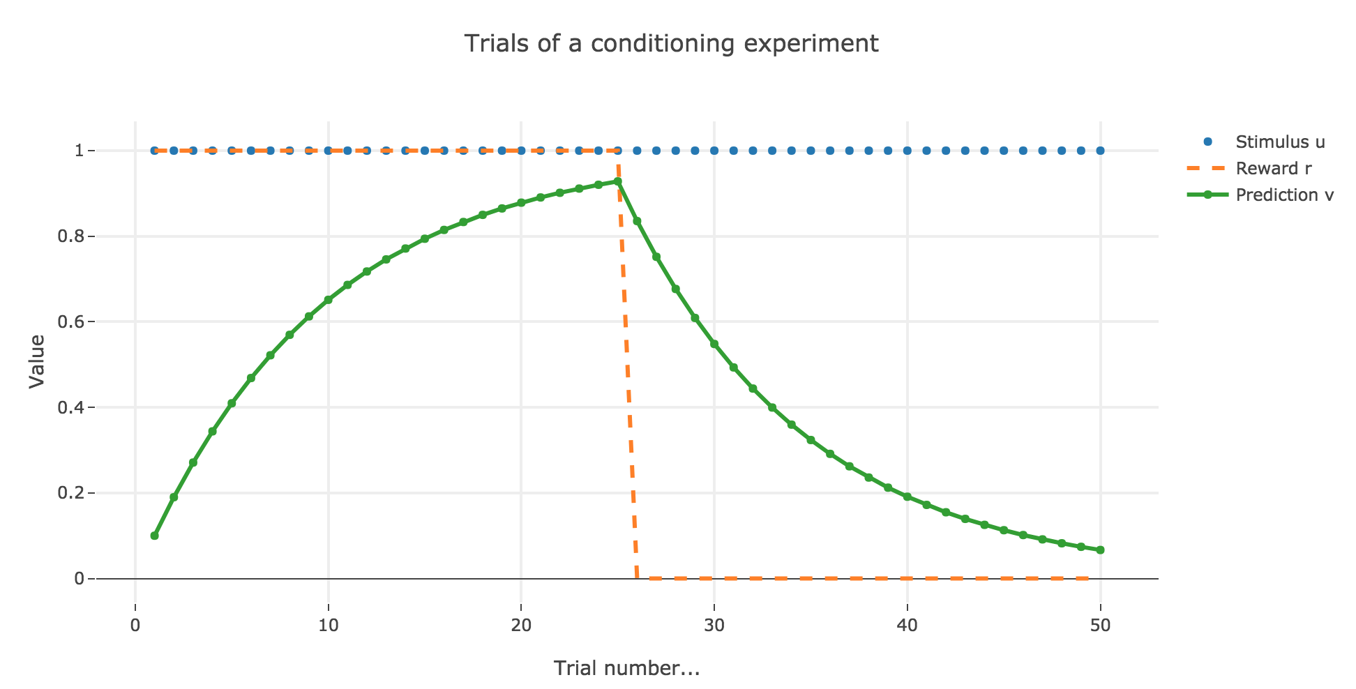
where the learning rate $ε$ is set to be $0.1$.
It appears that the animal prediction $v = wu$ does tend toward the reward. Indeed, if $r_i ≝ r_0$ and $u_i ≝ u_0$ are constant (as it happens here for the first $25$ trials, and for the last $25$ ones):
\[\begin{align*} w_{i+1} & = w_i + ε (r_0 − u_0 w_i) u_0 \\ & = (1- ε u_0^2) w_i + ε r_0 u_0 \\ \end{align*}\]Therefore:
\[\begin{align*} ∀i ≥ i_0, \; w_i &= (1- ε u_0^2)^{i-i_0} \Big(w_{i_0} - \frac{ε r_0 u_0}{1-(1-ε u_0^2)}\Big) + \frac{ε r_0 u_0}{1-(1-ε u_0^2)}\\ &= \frac{r_0}{u_0}\Big(1 - (1-ε u_0^2)^{i-i_0}\Big) + w_{i_0} (1-ε u_0^2)^{i-i_0} \\ \end{align*}\]As a result:
-
for the first $25$ trials: $r_0 = u_0 = 1$ and $w_0 = i_0 = 0$, so that:
\[∀ i ∈ \lbrace 0, 24 \rbrace, \; w_i = 1 - (1-ε)^i \xrightarrow[i \to +∞]{} 1 = r_0\] -
for the last $25$ trials: $r_0 = 0, \; u_0 = 1$ and $i_0 = 24, \, w_{24} > 0$, so that:
\[∀ i ∈ \lbrace 25, 50 \rbrace, \; w_i = w_{24} (1-ε)^{i-24} \xrightarrow[i \to +∞]{} 0 = r_0\]
Changing the learning parameter $ε$
Now, let us change the learning rate $ε$ in the previous example.
For $ε ≤ 1$
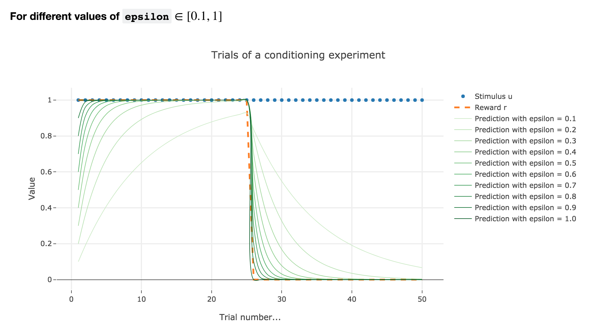
As illustrated by the figure above, when $ε ≤ 1$: the bigger the learning rate $ε$, the faster the animal prediction converges toward the reward.
Indeed, as shown above:
\[\begin{cases} ∀ i ∈ \lbrace 0, 24 \rbrace, \; w_i = 1 - (1-ε)^i \\ ∀ i ∈ \lbrace 25, 50 \rbrace, \; w_i = w_{24} (1-ε)^{i-24} \end{cases}\]so the bigger the learning rate $ε$, the lower the term $γ ≝ (1-ε)$, and the faster
- $w_i = 1 - γ^i$ converges toward the reward $1$ for the first $25$ trials
- $w_i = w_{24} γ^{i-24}$ converges toward the reward $0$ for the last $25$ trials
It can easily be shown that this observation holds for any constant piecewise reward.
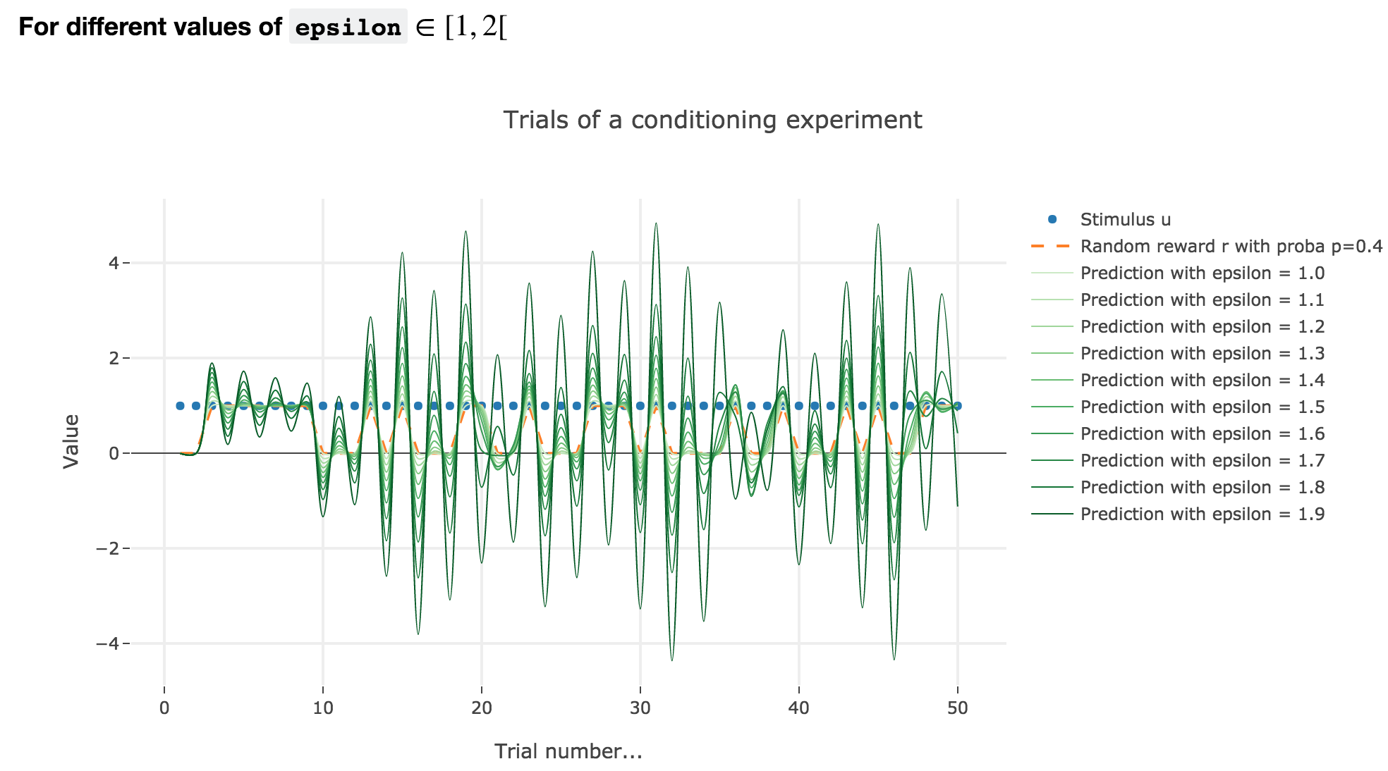
For $ε ∈ [1, 2[$
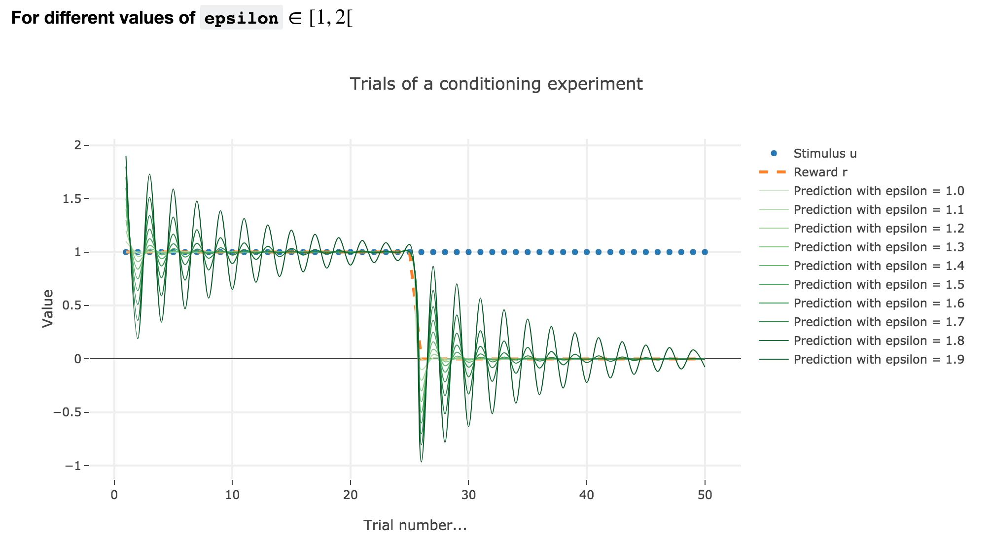
Analogously, if $ε ∈ [1, 2[$: the term $γ ≝ (1-ε) ∈ ]-1, 0]$, and for the first (resp. last) $25$ trials: $w_i = 1 - γ^i$ (resp. $w_i = w_{24} γ^{i-24}$) converges toward the reward $1$ (resp. $0$) while oscillating around it (since $γ ≤ 0$). The oscillation amplitude is all the more significant that $\vert γ \vert$ is big, i.e. that $ε$ is big.
Again, this result can be extended to any constant piecewise reward.
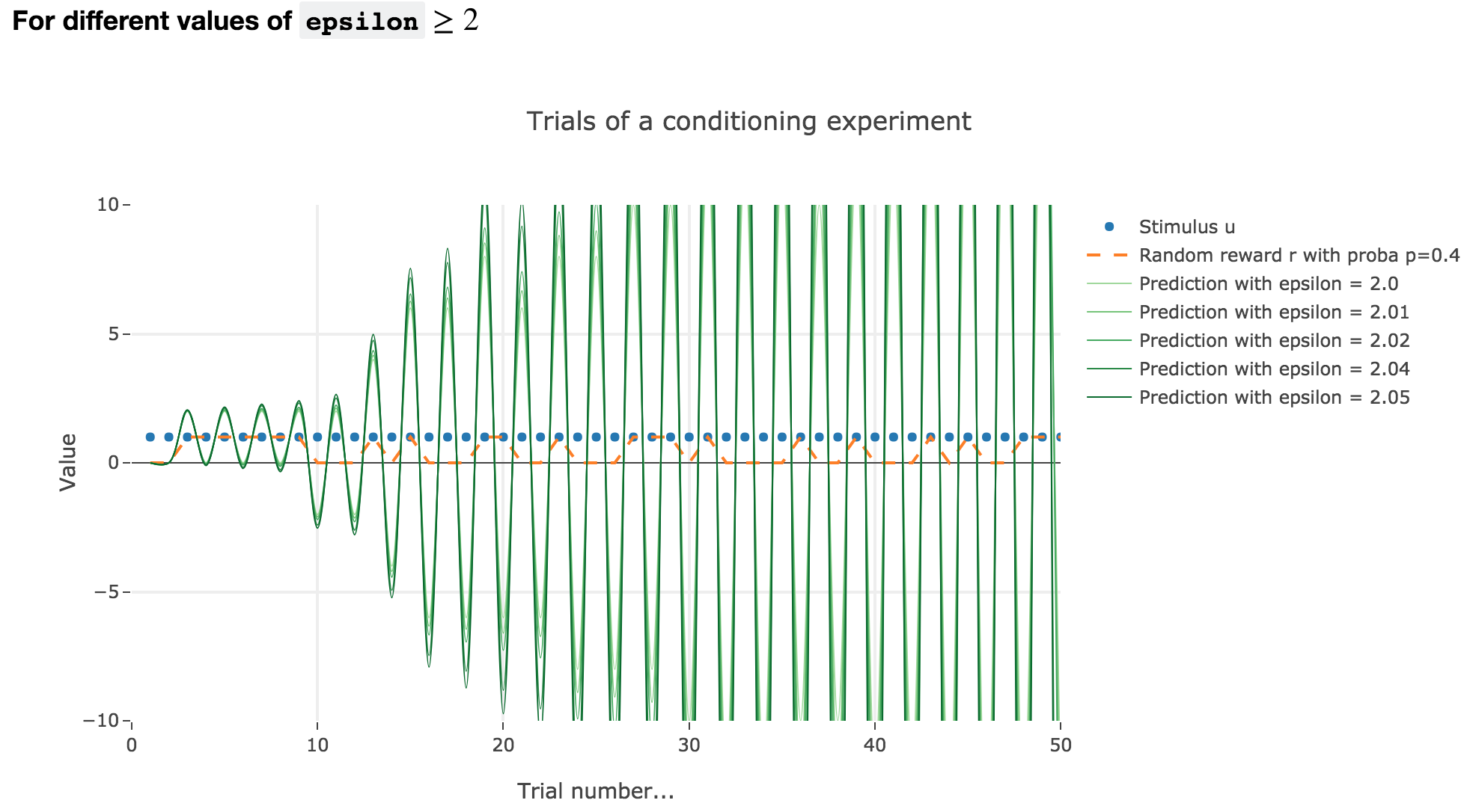
For $ε ≥ 2$
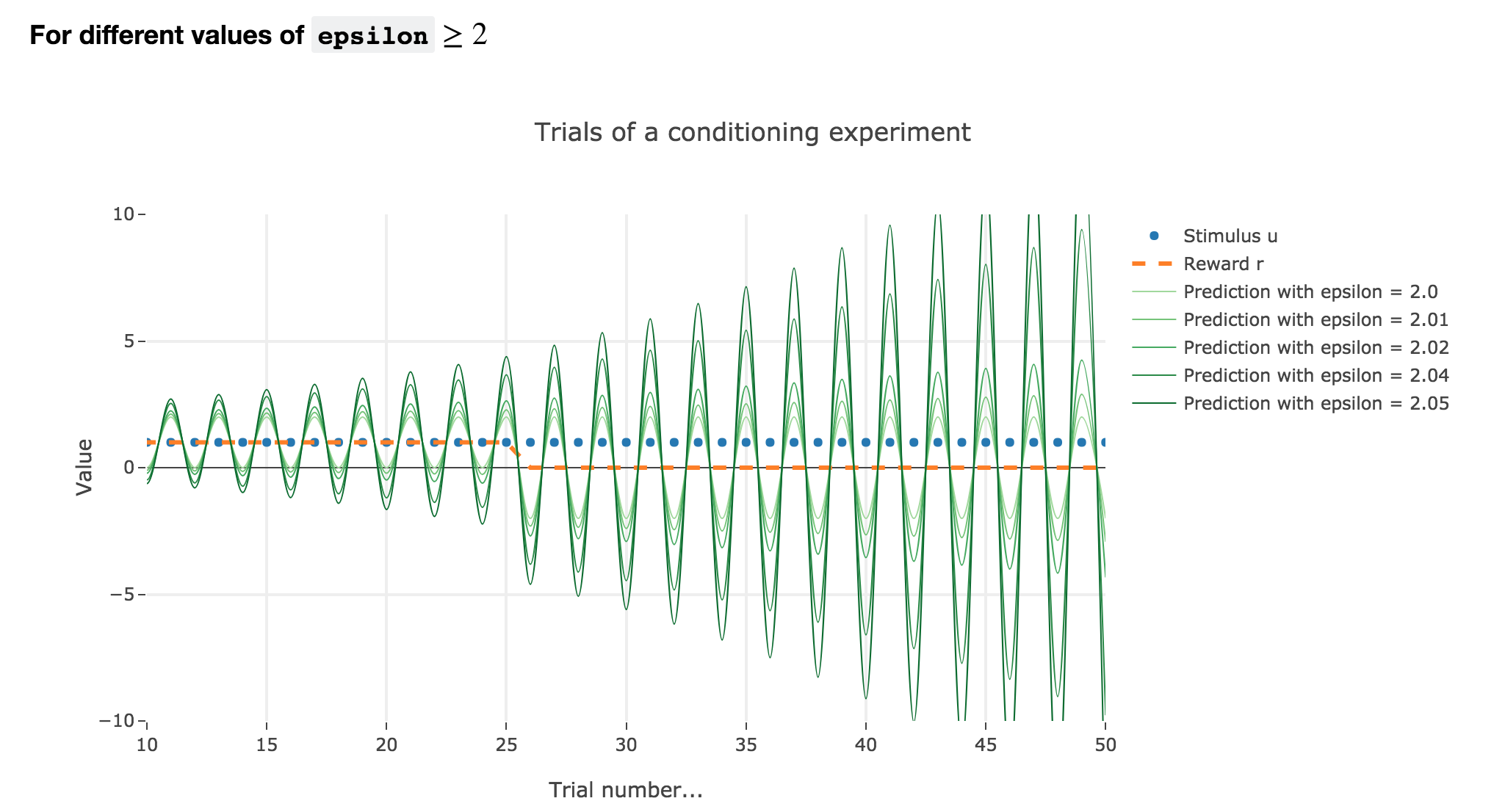
Finally, if $ε ≥ 2$: the term $γ ≝ (1-ε) ≤ -1$, and $w_i$ diverges as $γ^i$ does, while oscillating around it (since $γ ≤ 0$). The oscillation amplitude is all the more significant that $\vert γ \vert$ is big, i.e. that $ε$ is big.
Again, this result stands for any constant piecewise reward.
Going back to our conditioning experiment:
$ε ≤ 1$ corresponds to what is expected from the experiments: the bigger the learning rate, the faster the convergence of the animal prediction, monotonously for a constant reward: hence the name learning rate.
$ε ∈ [1 , 2[$ and $ε ≥ 2$ are both degenerate cases: $ε ≥ 2$ is completely nonsensical from a biological standpoint, and the oscillations of $ε ∈ [1 , 2[$ are not what we want to model, which is rather a convergence of the animal prediction straight to the reward.
2. Partial conditioning
Let us suppose that in each trial, the stimulus is present, but the presence of the reward is a random event with probability $0.4$.
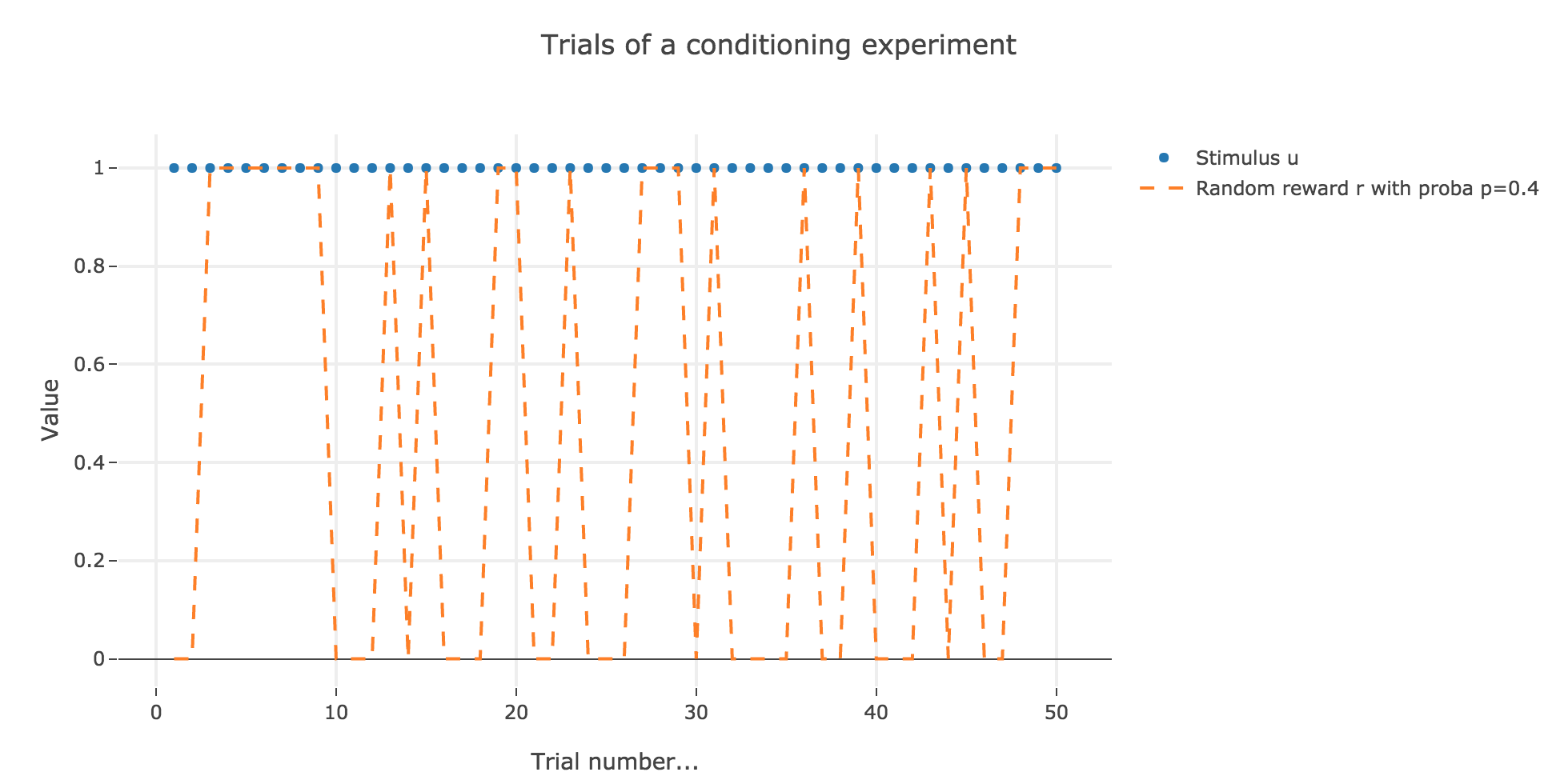
Similarly to what has been done in the previous section:
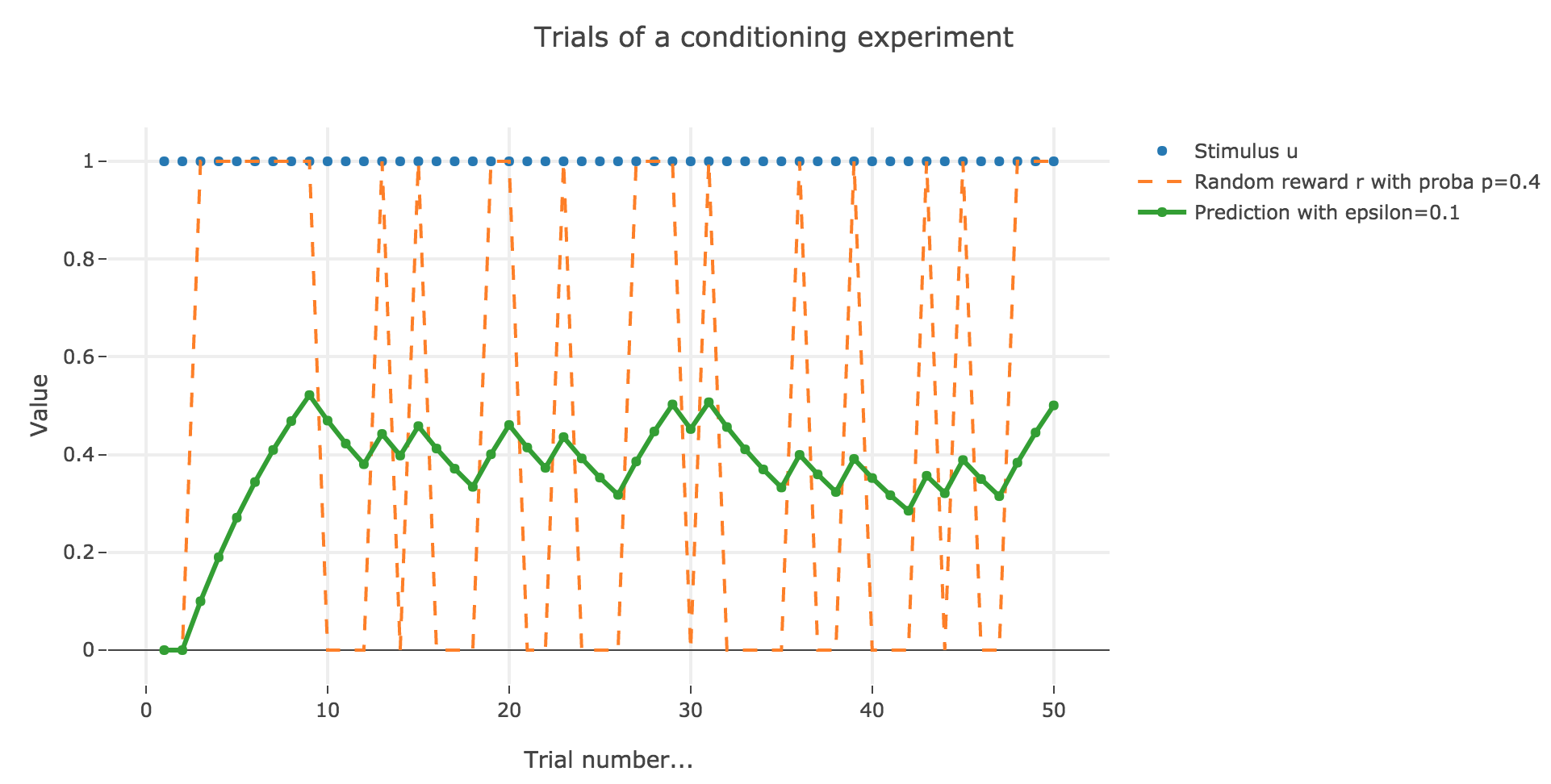
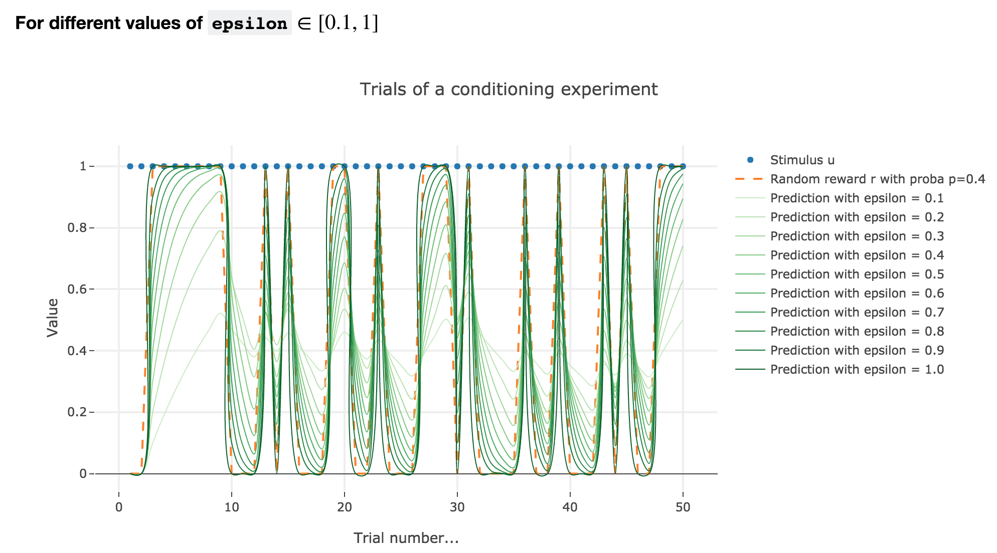
As it happens, the reward is a constant piecewise function, so the previous analysis applies here, by focusing on each segment where the reward is constant (the stimulus is always equal to $1$ here, which simplifies things up). On top of that, we may stress that the shorter these segments are, the higher $ε ≤ 1$ has to be, for the animal to learn the reward within these shorter time spans. The oscillating cases are still irrelevant from a biological standpoint.
3. Blocking
Now, we assume that there are two stimuli, $u_1$ and $u_2$, and two parameters, $w_1$ and $w_2$ to learn, and that the animal prediction is given by $v = w_1 u_1 + w_2 u_2$.
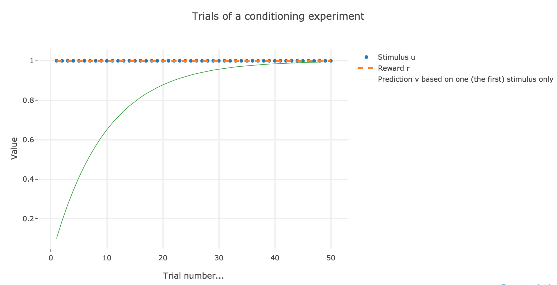
During the first $25$ trials, only one stimulus and the reward are present, during the next $25$ trials, both stimuli and the reward are present.
For the record, here is what happens when there is one single stimulus and $u = r = 1$:
Now, with aforementioned two stimuli:
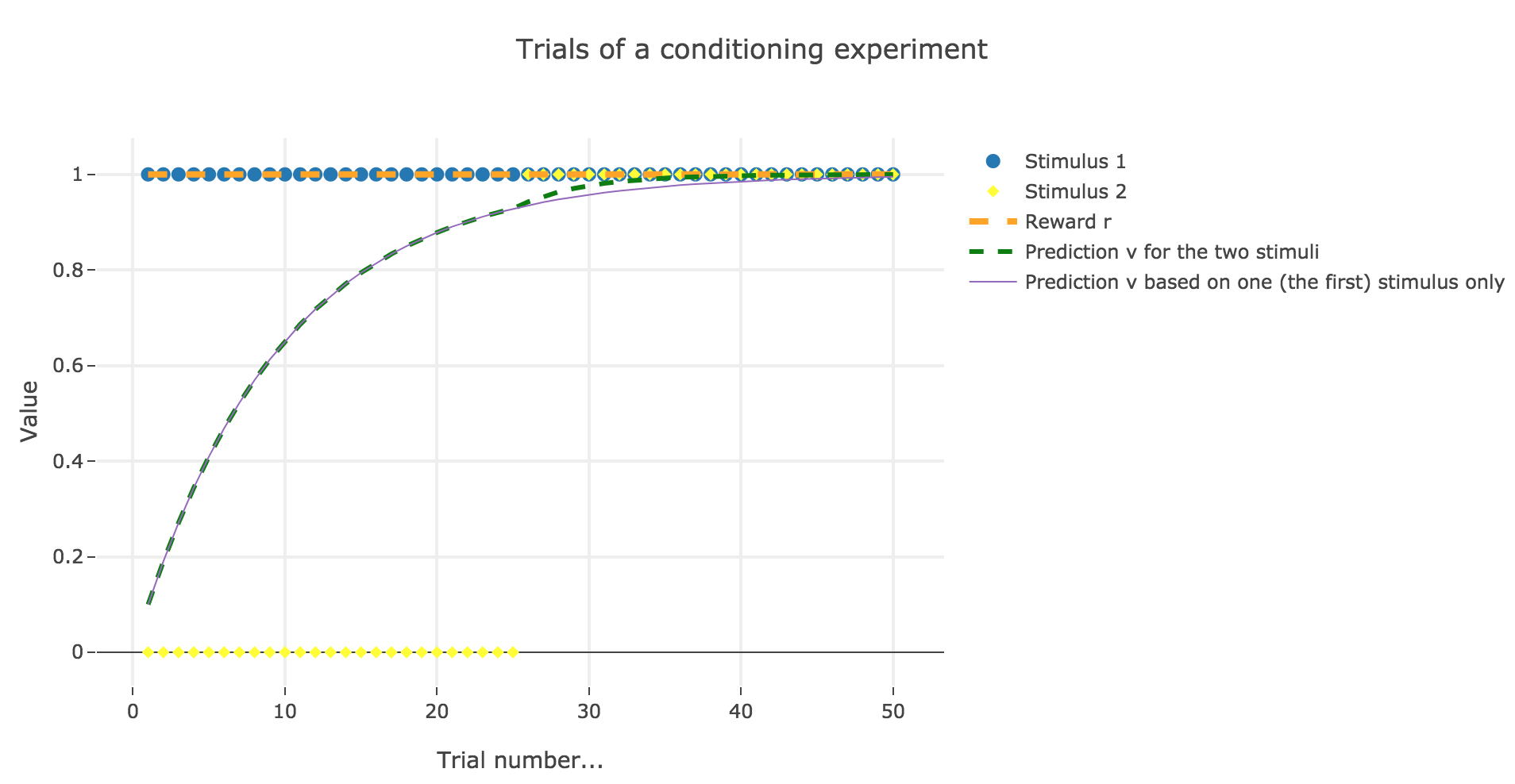
To be more precise, here is the evolution of $w_1$ and $w_2$ throughout the trials:
| Trial | $w_1$ | $w_2$ |
|---|---|---|
| 1 | 0.1 | 0. |
| 2 | 0.19 | 0. |
| 3 | 0.271 | 0. |
| 4 | 0.3439 | 0. |
| 5 | 0.40951 | 0. |
| 6 | 0.468559 | 0. |
| 7 | 0.5217031 | 0. |
| 8 | 0.56953279 | 0. |
| 9 | 0.61257951 | 0. |
| 10 | 0.65132156 | 0. |
| 11 | 0.6861894 | 0. |
| 12 | 0.71757046 | 0. |
| 13 | 0.74581342 | 0. |
| 14 | 0.77123208 | 0. |
| 15 | 0.79410887 | 0. |
| 16 | 0.81469798 | 0. |
| 17 | 0.83322818 | 0. |
| 18 | 0.84990536 | 0. |
| 19 | 0.86491483 | 0. |
| 20 | 0.87842335 | 0. |
| 21 | 0.89058101 | 0. |
| 22 | 0.90152291 | 0. |
| 23 | 0.91137062 | 0. |
| 24 | 0.92023356 | 0. |
| 25 | 0.9282102 | 0. |
| 26 | 0.93538918 | 0.00717898 |
| 27 | 0.94113237 | 0.01292216 |
| 28 | 0.94572691 | 0.01751671 |
| 29 | 0.94940255 | 0.02119235 |
| 30 | 0.95234306 | 0.02413286 |
| 31 | 0.95469547 | 0.02648527 |
| 32 | 0.95657739 | 0.02836719 |
| 33 | 0.95808294 | 0.02987273 |
| 34 | 0.95928737 | 0.03107717 |
| 35 | 0.96025092 | 0.03204071 |
| 36 | 0.96102175 | 0.03281155 |
| 37 | 0.96163842 | 0.03342822 |
| 38 | 0.96213176 | 0.03392156 |
| 39 | 0.96252643 | 0.03431623 |
| 40 | 0.96284216 | 0.03463196 |
| 41 | 0.96309475 | 0.03488455 |
| 42 | 0.96329682 | 0.03508662 |
| 43 | 0.96345848 | 0.03524827 |
| 44 | 0.9635878 | 0.0353776 |
| 45 | 0.96369126 | 0.03548106 |
| 46 | 0.96377403 | 0.03556383 |
| 47 | 0.96384024 | 0.03563004 |
| 48 | 0.96389321 | 0.03568301 |
| 49 | 0.96393559 | 0.03572539 |
| 50 | 0.96396949 | 0.03575929 |
There is a phenomenon of blocking in the sense that: when $u_2$ appears (from the trial $26$ on), the prediction error is already close to zero (the animal has already almost exclusively associated the presence of the reward with the presence of the first stimulus only), so that the second stimulus is hardly taken into account, compared to the first one (hence the blocking).
4. Overshadowing
We still suppose that there are two stimuli and two parameters to learn. However, now:
-
both stimuli and the reward are present throughout all the trials.
-
one of the learning rates is larger: $ε_1 = 0.2$ for the first stimulus, and $ε_2 = 0.1$ for the other one
Here is the evolution of $w_1$ and $w_2$ throughout the trials:
| Trial | $w_1$ | $w_2$ |
|---|---|---|
| 1 | 0.2 | 0.1 |
| 2 | 0.34 | 0.17 |
| 3 | 0.438 | 0.219 |
| 4 | 0.5066 | 0.2533 |
| 5 | 0.55462 | 0.27731 |
| 6 | 0.588234 | 0.294117 |
| 7 | 0.6117638 | 0.3058819 |
| 8 | 0.62823466 | 0.31411733 |
| 9 | 0.63976426 | 0.31988213 |
| 10 | 0.64783498 | 0.32391749 |
| 11 | 0.65348449 | 0.32674224 |
| 12 | 0.65743914 | 0.32871957 |
| 13 | 0.6602074 | 0.3301037 |
| 14 | 0.66214518 | 0.33107259 |
| 15 | 0.66350163 | 0.33175081 |
| 16 | 0.66445114 | 0.33222557 |
| 17 | 0.6651158 | 0.3325579 |
| 18 | 0.66558106 | 0.33279053 |
| 19 | 0.66590674 | 0.33295337 |
| 20 | 0.66613472 | 0.33306736 |
| 21 | 0.6662943 | 0.33314715 |
| 22 | 0.66640601 | 0.33320301 |
| 23 | 0.66648421 | 0.3332421 |
| 24 | 0.66653895 | 0.33326947 |
| 25 | 0.66657726 | 0.33328863 |
| 26 | 0.66660408 | 0.33330204 |
| 27 | 0.66662286 | 0.33331143 |
| 28 | 0.666636 | 0.333318 |
| 29 | 0.6666452 | 0.3333226 |
| 30 | 0.66665164 | 0.33332582 |
| 31 | 0.66665615 | 0.33332807 |
| 32 | 0.6666593 | 0.33332965 |
| 33 | 0.66666151 | 0.33333076 |
| 34 | 0.66666306 | 0.33333153 |
| 35 | 0.66666414 | 0.33333207 |
| 36 | 0.6666649 | 0.33333245 |
| 37 | 0.66666543 | 0.33333271 |
| 38 | 0.6666658 | 0.3333329 |
| 39 | 0.66666606 | 0.33333303 |
| 40 | 0.66666624 | 0.33333312 |
| 41 | 0.66666637 | 0.33333318 |
| 42 | 0.66666646 | 0.33333323 |
| 43 | 0.66666652 | 0.33333326 |
| 44 | 0.66666656 | 0.33333328 |
| 45 | 0.6666666 | 0.3333333 |
| 46 | 0.66666662 | 0.33333331 |
| 47 | 0.66666663 | 0.33333332 |
| 48 | 0.66666664 | 0.33333332 |
| 49 | 0.66666665 | 0.33333332 |
| 50 | 0.66666665 | 0.33333333 |
There is a phenomemon of overshadowing: the first stimulus ends up being taken into account twice as much as the second (overshadowing it), as it has been learned at a rate two times bigger.
PROBLEM 2: Simple decision strategy for flower sampling by bees.
Link of the iPython notebook for the code
Let us consider the following experiment: a bee lands on flowers to collect as much nectar as possible, during two day (granting that it lands on $100$ flowers a day). There are two kinds of flowers:
-
blue flowers, which carry a nectar reward of
- $r_b = 8$ during the first day
- $r_b = 2$ during the second day
-
yellow flowers, which carry a nectar reward of
- $r_y = 2$ during the first day
- $r_y = 8$ during the second day
The bee’s internal estimate for the rewards is $m_b$ (resp. $m_y$) for the blue (resp. yellow) flowers. The bee chooses to land on a blue flower with probability (softmax-strategy):
\[p_b = \frac{1}{1 + \exp(β (m_y - m_b))}\]where $β$ is called the “exploitation-exploration trade-off” parameter (we will explain why in the following section).
1. The softmax-strategy
Note that $p_b$ is a sigmoid of $-(m_y - m_b)$ (for a fixed $β$) and a sigmoid of $-β$ (for a fixed $m_y - m_b$).
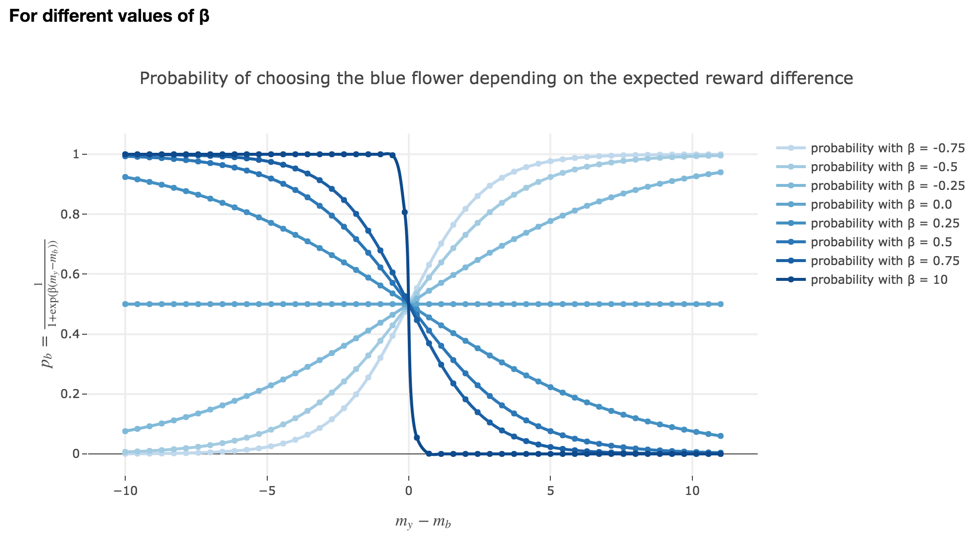
Thus:
-
the larger $m_y - m_b$, the higher the bee’s internal estimate of the yellow flower is compared to the blue one. As a consequence, the lower the probability $p_b$ of the bee landing on the blue one.
-
the lower the reward difference, the worse the bee considers the yellow flower to be, compared to the blue one, and the greater the probability $p_b$ of the bee landing on the blue flower.
-
in between: the bee’s behavior is a mix between exploiting what the bee deems to be the most nutritious flower and exploring the other one (which is what is expected).
Symetrically:
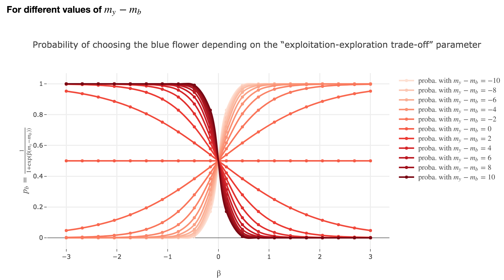
The “exploitation-exploration trade-off” parameter $β$
For $β ≥ 0$
As seen in the previous figures: the parameter $β$ plays the same role as the inverse temperature $β ≝ \frac{1}{k_B T}$ in statistical physics. That is, for $β ≥ 0$:
-
When $β ⟶ +∞$: the bigger $β$ is (which corresponds, in physics, to a low temperature/entropy), the more the bee tends to exploit the seemingly most nutritious flower. As a result:
- if $m_y-m_b > 0$ (i.e. the yellow flower seems more avantageous to the bee), the probability of the bee landing on the blue flower rapidly decreases to $0$
- if $m_y-m_b < 0$ (i.e. the blue flower seems more advantageous to the bee), the probability of the bee landing on the blue flower rapidly increases to $1$
-
When $β ⟶ 0$: the lower $β$ is (high temperature/entropy in physics), the more the bee tends to explore the flowers.
Indeed: as $β ⟶ 0$, $p_b$ becomes less and less steep, to such a point that it ends up being the constant function $1/2$ when $β=0$ (at this point, the bee does nothing but exploring, since landing on either of the flowers is equiprobable, no matter how nutritious the bee deems the flowers to be)
For $β < 0$
As
\[p_b(-β, m_y-m_b) = \frac{1}{1 + \exp(-β (m_y-m_b))} = \frac{1}{1 + \exp(β (-(m_y-m_b)))} = p_b(β, -(m_y-m_b))\]The curves for $-β < 0$ are symmetric to those for $β > 0$ with respect to the y-axis, which makes no sense from a behavioral point of vue: it means that the most nutritious a flower appears to the bee, the less likely the bee is to land on it (and conversely)!
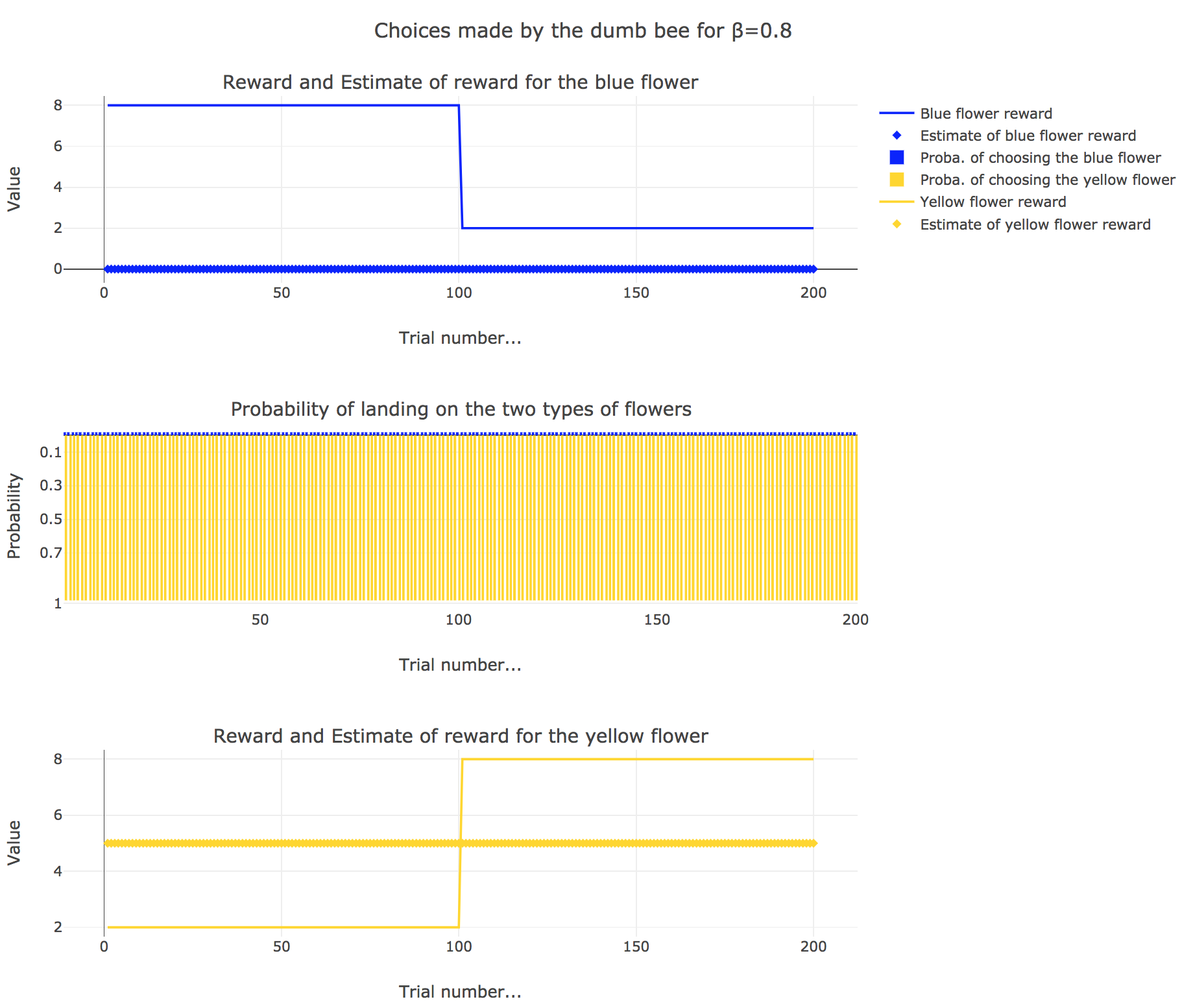
2. Dumb bee
Now, let us assume that the bee is “dumb”, i.e. it does not learn from experience: throughout all the trials, the internal reward estimates remain constant: $m_y = 5, \; m_b = 0$.
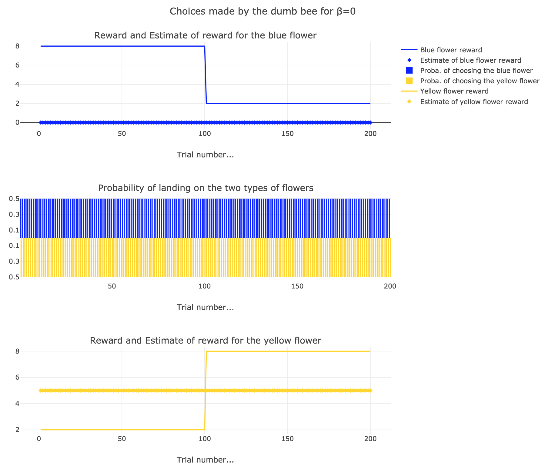
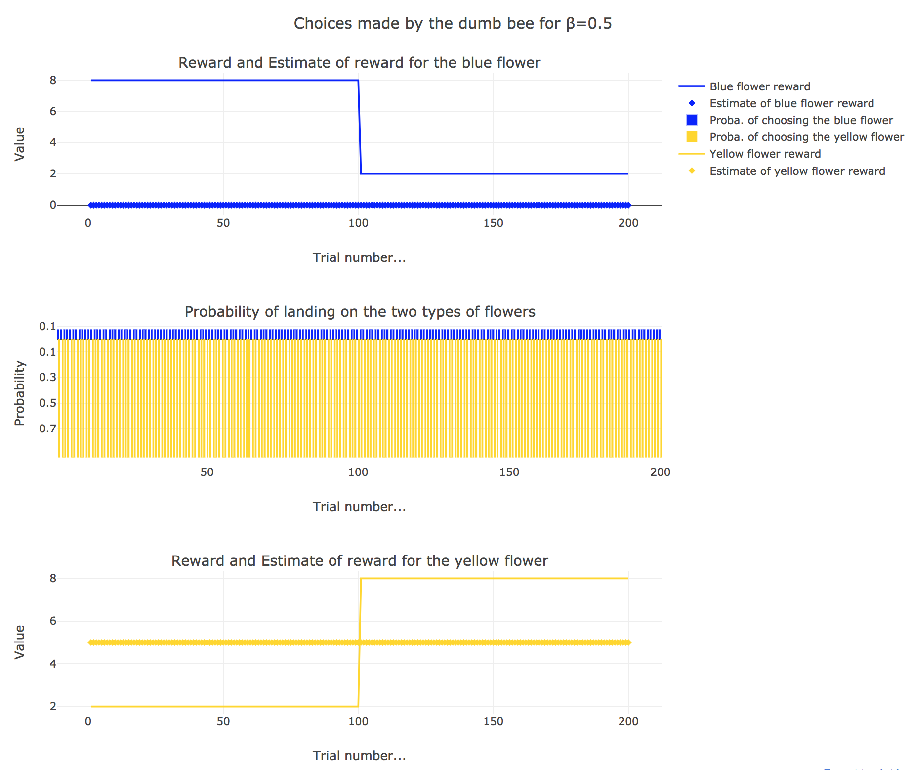
So it appears that
-
for $β = 0$: the bee’s behavior is the most exploratory one: the probability of landing on a blue flower as well as a yellow flower is $1/2$, irrespective of the internal estimates $m_b$ and $m_y$
-
for $β = 0.5$: this $β$ corresponds to a perfectly balanced exploration-exploitation tradoff, but here: as $m_y = 5$ is significantly higher that $m_b = 0$, $p_y ≝ 1-p_b » p_b$ (which are constant, as the internal estimates are constant)
-
for $β = 1$: the bee’s behavior is the most exploitative one. As $m_y > m_b$, $p_y ≃ 1$: the bee keep exploiting the flower it deems the most nutritious (i.e. the yellow ones).
On the whole, this behavior can reasonably be called “dumb”, since the bee takes no account of the actual rewards of the flowers whatsoever (its internal estimates remain constant and don’t depend on these actual rewards).
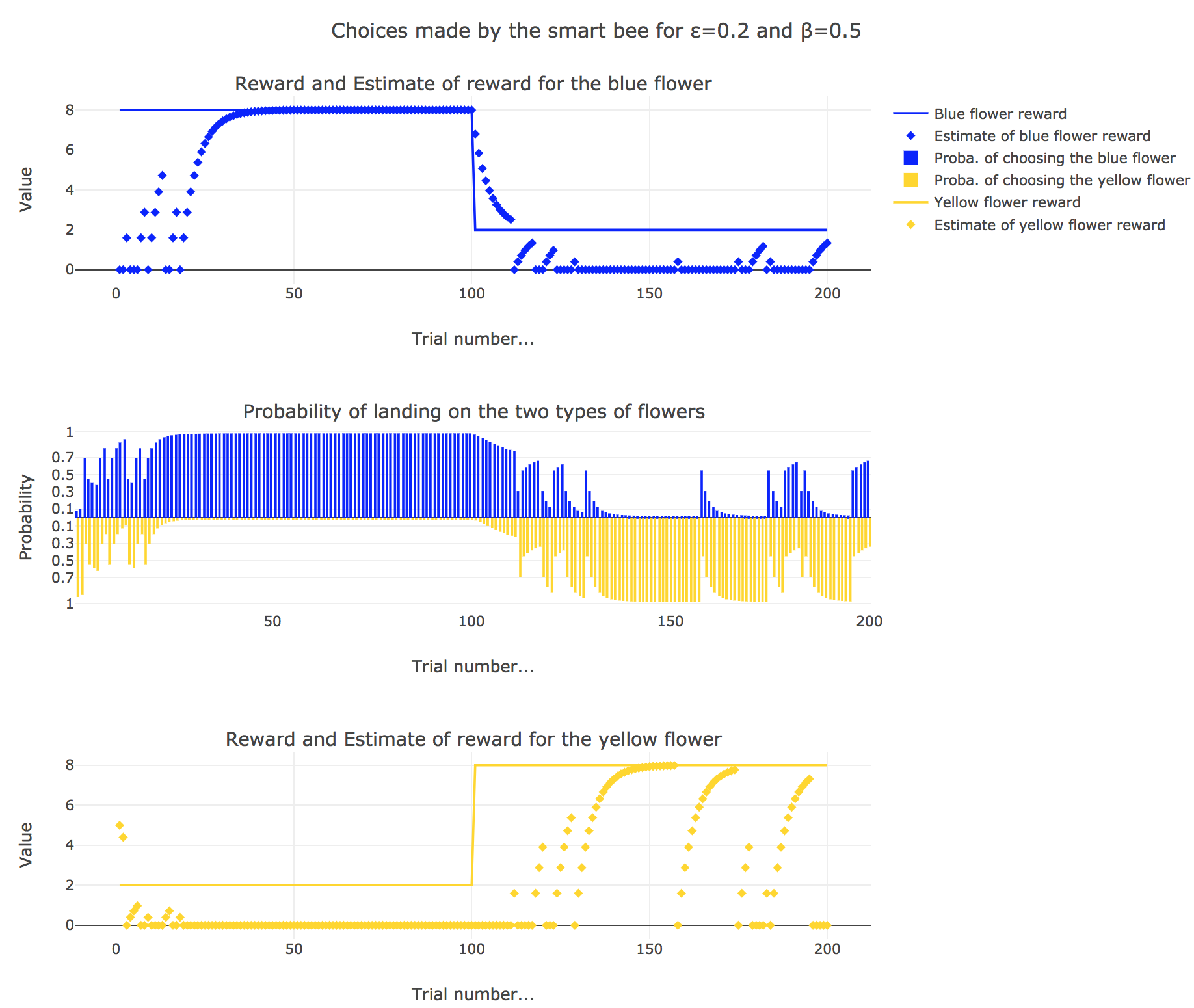
3. Smart bee
Now let us suppose that the bee is “smart”, i.e. it can learn from its experiences. Whenever it visits a flower, it updates its estimated reward as follows:
\[\begin{align*} m_b &→ m_b + ε(r_b − m_b)\\ m_y &→m_y +ε(r_y − m_y) \end{align*}\]Given a learning parameter $ε = 0.2$ and the initial assumptions about flower reward from above ($m_y = 5, m_b = 0$), simulate the bees sequence of choices during the two days. How do the reward estimates change over time? Explore the case of purely explorative behavior ($β = 0$) and the case of strongly exploitative behavior ($β = 1$). What do you observe?
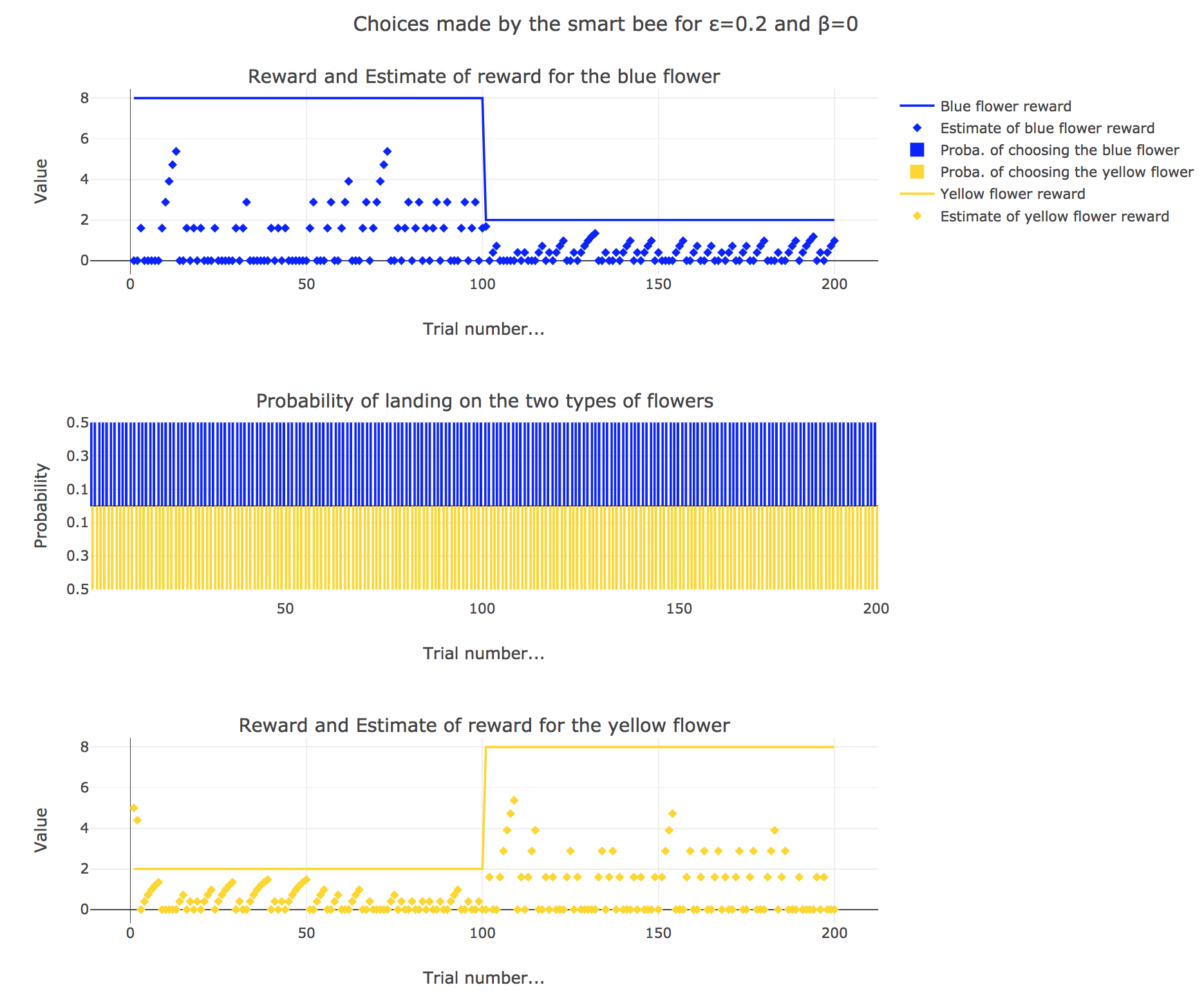
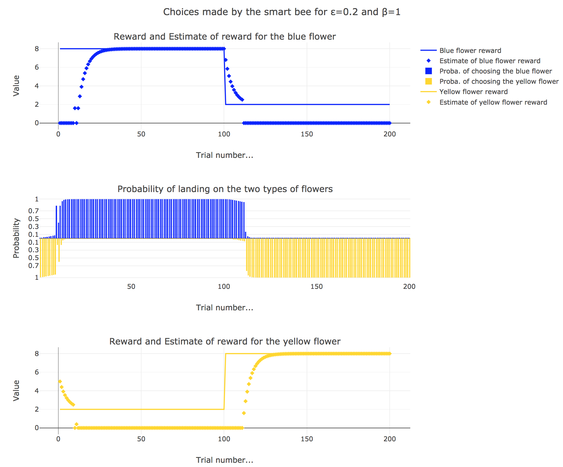
It appears that
-
for $β = 0$: no surprise, the bee’s behavior is the most exploratory one: the probability of landing on a blue flower as well as a yellow flower is $1/2$, irrespective of the internal estimates $m_b$ and $m_y$
-
for $β = 1$: the bee’s behavior is the most exploitative one. Similarly to the Rescola-Wagner rule, the updating rule makes the internal estimates converge toward the actual rewards of the flowers, and as result: the exploitative behavior causes the probability $p_b$ (resp. $p_y ≝ 1-p_b$) to match the evolution of the internal estimate $m_b$ (resp. $m_y$) when $m_b > m_y$ (resp. $m_y > m_b$): the bee exploit the flower type which has the highest current estimate.
-
for $β = 0.5$: it is a mixed behavior bewteen exploitation and exploration: compared to the case $β=1$, there are some discrepancies in the update of the internal estimates, since the bee may not always exploit the flower type which has the best current estimate (exploratory behavior).
On the whole, this behavior can reasonably be called “smart”, since the bee, depending on the value of $β$:
takes more or less into account the actual rewards of the flowers by exploiting the seemingly most nutritious flower (exploitation, increasing with $β$)
while, from time to time, completely ignoring its internal estimates and exploring the other flower (exploration, decreasing with $β$)
PROBLEM 3: The drift diffusion model of decision-making.
Link of the iPython notebook for the code
We consider a two-alternative forced choice task (2AFC-task): the subject (e.g. a monkey) sees a cluster of moving dots (in many directions) on a screen and is to choose (whenever he/she/it wants) whether they are moving upwards or downwards.
In the drift-diffusion-model, the subject is assumed to compare two firing rates:
- one firing rate of an upward-motion sensitive neuron, denoted by $m_A$
- and another one from a downward-motion sensitive neuron, denoted by $m_B$
Then, the subjects integrates the difference as follows:
\[\dot{x} = m_A − m_B + σ η(t)\]where $η(t) \sim 𝒩(0, 1)$ is a Gaussian white noise.
For a given threshold $μ$:
- if $x ≥ μ$ then the subject chooses $A$
- else if $x ≤ -μ$ then the subject chooses $B$
We have the following discrete approximation of the drift-diffusion-model:
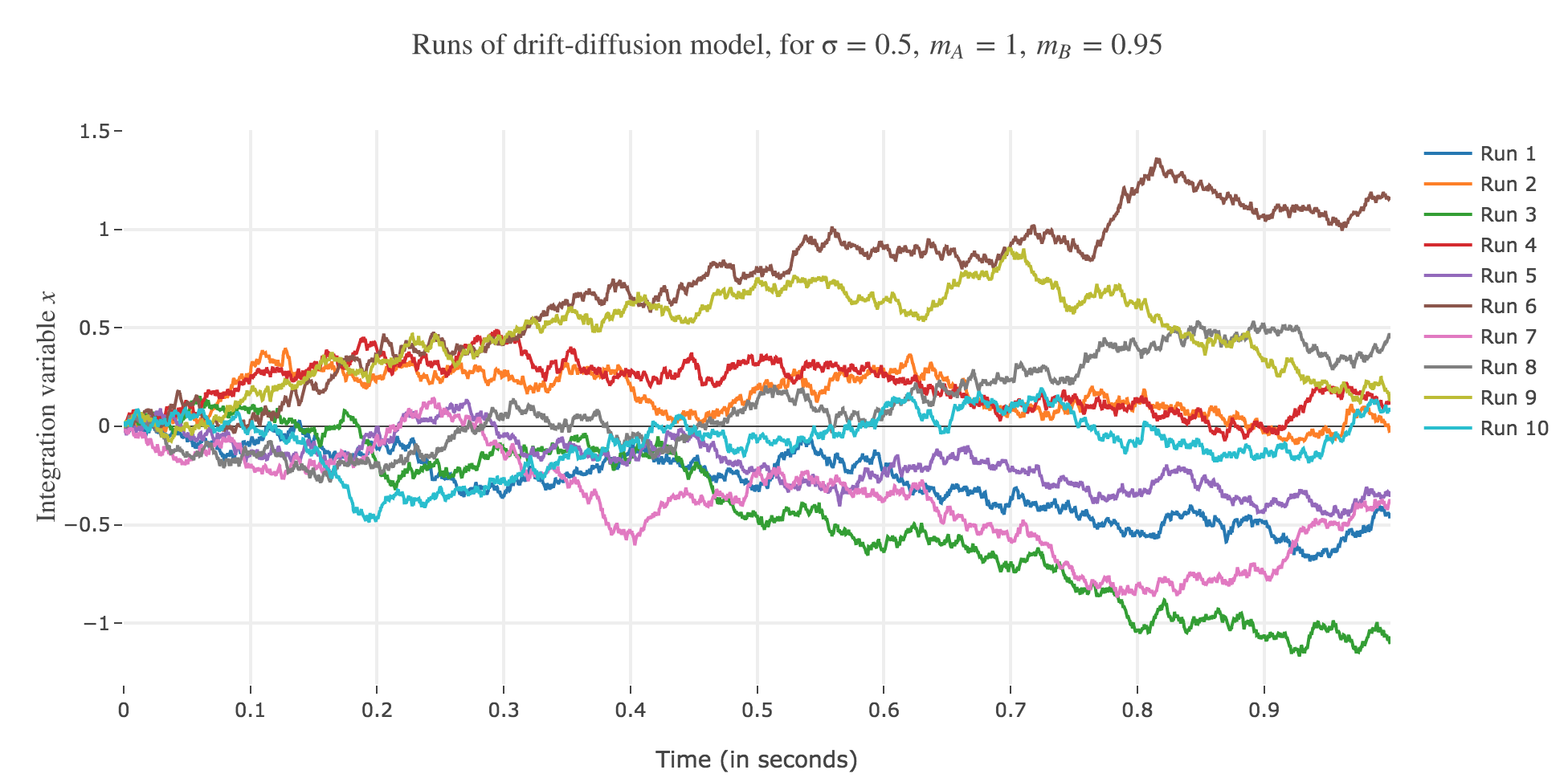
\[x(t+∆t) = x(t) + (m_A - m_B) ∆t + σ η(t) \sqrt{∆t}\]1. Reaction times
Let $m_A ≝ 1, m_B ≝ 0.95, \, σ ≝ 0.5, \, x(0) ≝ 0$, and $∆t ≝ 0.1 \, \mathrm{ ms}$.
Let us run the drift-diffusion-model ten times with the above parameters, with resort to the Euler method:
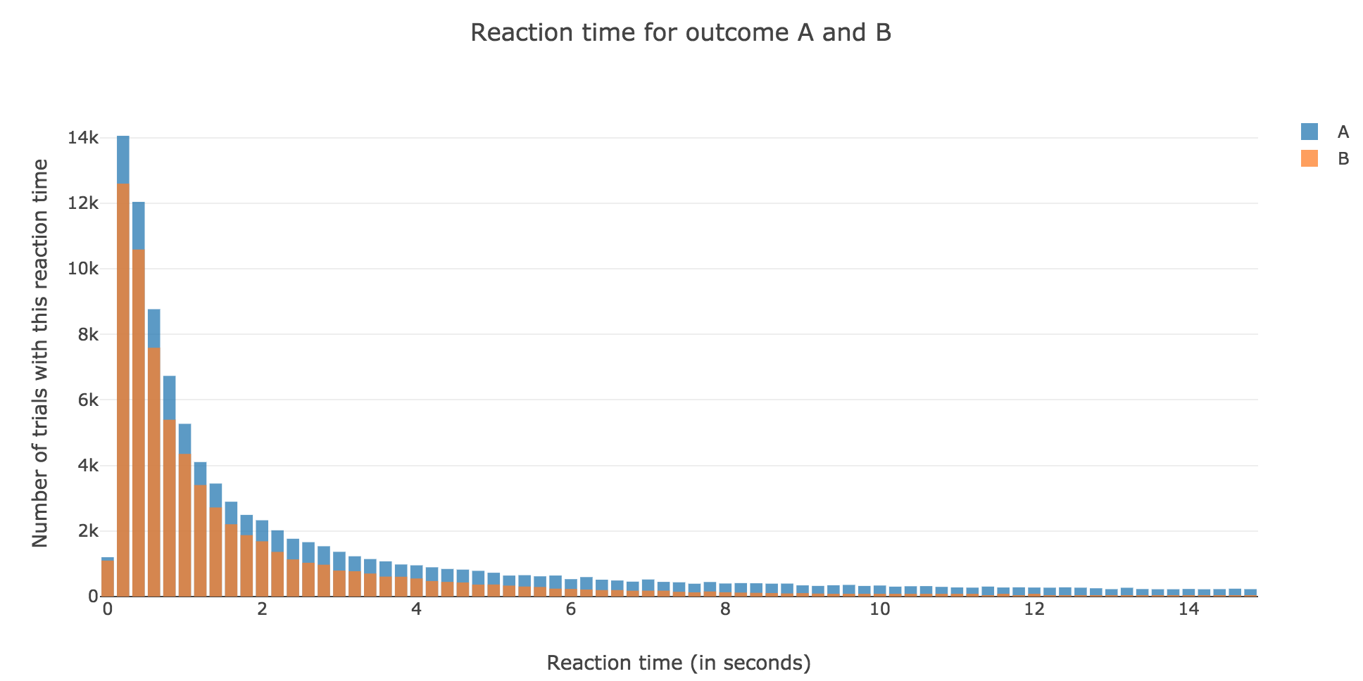
Now, after running the model $N$ times and storing the outcome and the time of threshold crossing (denoted by $t_i$) for each run: let us plot the distribution of reaction times for outcome $A$ and $B$, given that the reaction time is given by:
\[RT_i = 100 + t_i\]-
For $N ≝ 1000$:
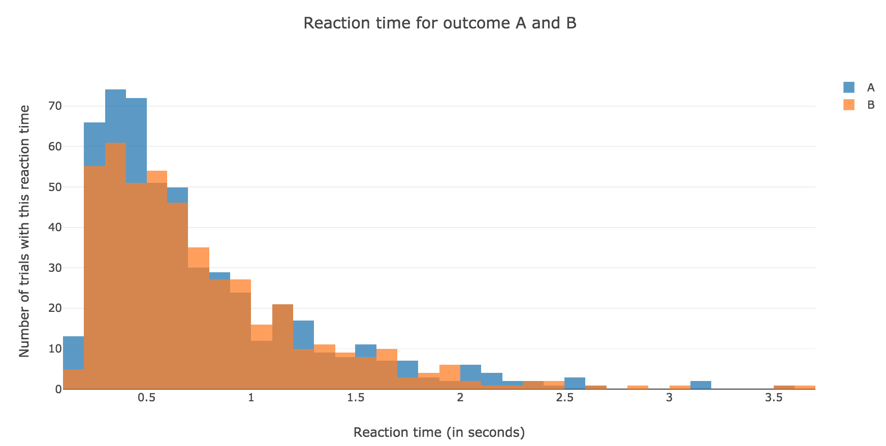
Figure 1.1. - Distribution of reaction times for outcome $A$ and $B$ after running the model $N = 1000$ times -
For $N ≝ 10000$:
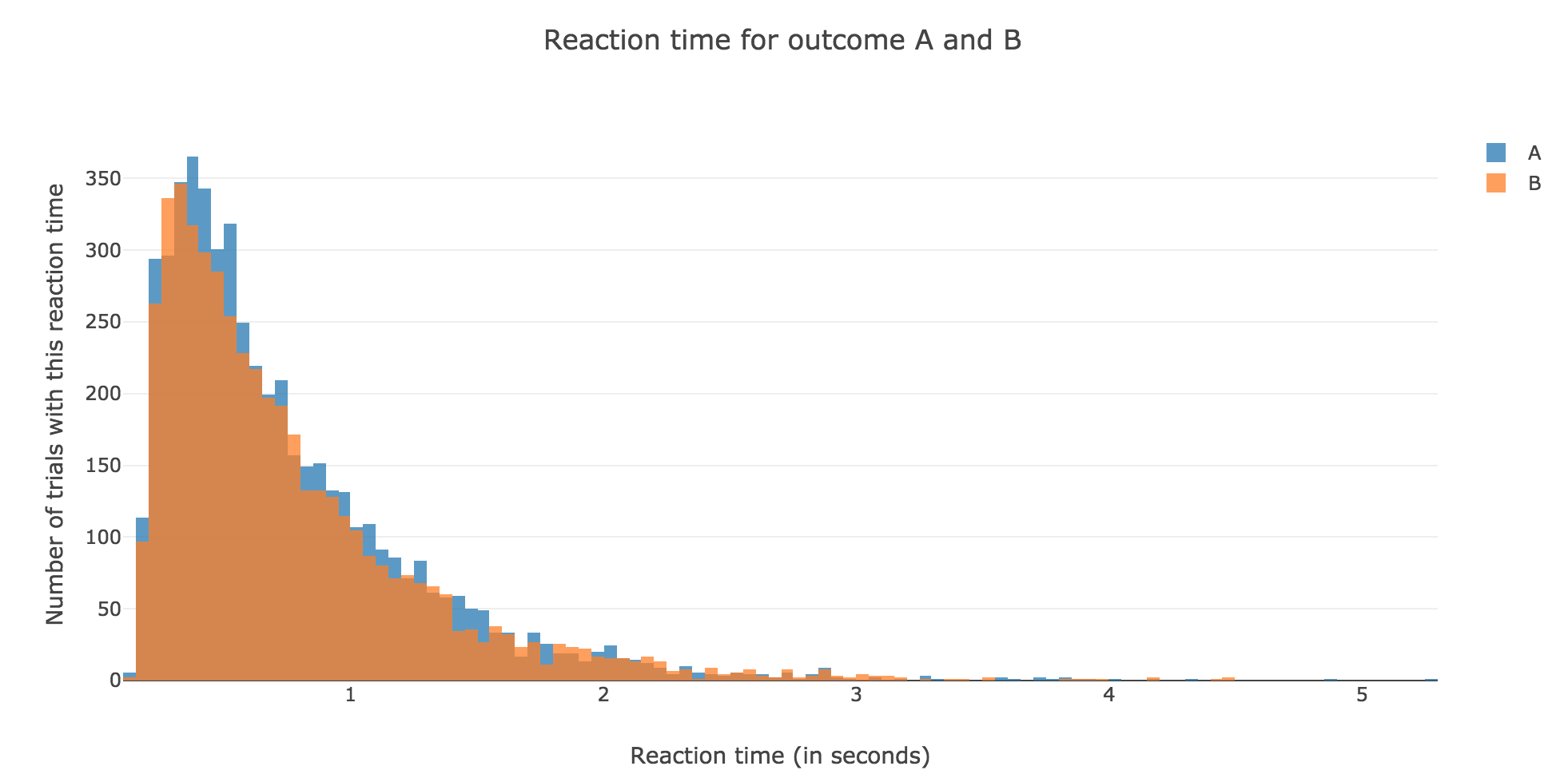
Figure 1.2. - Distribution of reaction times for outcome $A$ and $B$ after running the model $N = 10000$ times
2. Probability of outcome $A$
Let us define the evidence for outcome $A$ versus outcome $B$ as:
\[m_E ≝ m_A - m_B\]The analytical formula of the probability of outcome $A$ is:
\[p_A ≝ \frac{1}{1+ \exp(-β m_E)}\]where $β ≝ \frac{2 μ}{σ^2}$.
Let us compare it, for values of $m_E$ ranging from $-0.2$ to $0.2$, with the empirical probability we can get from our simulation, by running the model $N$ times (for $N$ sufficiently large) and computing:
\[P(A) ≝ \frac{\text{Number of trials of outcome } A}{\text{Number of trials of outcome } A + \text{Number of trials of outcome } B}\]The problem is that we have to compute this empirical probability for several values of $m_E$ ranging from $-0.2$ to $0.2$! As a matter of fact: the previous naive algorithm, based on the Euler method, is far too slow…
But we can cope with that with a trick!
Fast algorithm to compute the distribution of reaction times
From the discrete approximation of the drift-diffusion-model:
\[x(t+∆t) = x(t) + m_E ∆t + σ η(t) \sqrt{∆t}\]So for all $n ≥ 1$:
\[x(t+ n ∆t) = x(0) + n \cdot m_E ∆t + σ \sqrt{∆t} \sum\limits_{ i=1 }^n η_i(t)\]where the
\[η_i(t) \sim 𝒩(\overbrace{0}^{ ≝ \, μ_i}, \overbrace{1}^{≝ \, σ_i^2})\]are independent and normally distributed random variables.
But it is well known that a sum of independent and normally distributed random variables is also a normally distributed variable, such that:
\[\sum\limits_{ i=1 }^n η_i(t) \sim 𝒩\left(\sum\limits_{ i=1 }^n μ_i \, , \; \sum\limits_{ i=1 }^n σ_i^2\right)\]i.e.
\[\sum\limits_{ i=1 }^n η_i(t) \sim 𝒩(0, n)\]But as it happens:
\[\sqrt{n} \underbrace{η(t)}_{\sim 𝒩(0, 1)} \sim 𝒩(0, n)\]So for all $n ≥ 1$, we can set $x(t + n ∆t)$ to be:
\[x(t + n ∆t) = x(0) + n \cdot m_E ∆t + \sqrt{n} \cdot σ \sqrt{∆t} η(t)\]where $η(t) \sim 𝒩(0, 1)$
So solving for $n$ in the threshold crossing conditions:
\[x(t + n ∆t) = ± μ\]is tantamount to:
-
Analysis: solving (for $ξ$, in $ℂ$) two quadratic equations for a given $η(t) ∈ ℝ$:
\[\begin{cases} m_E ∆t \, ξ^2 + σ \sqrt{∆t} η(t) \, ξ + x(0) - μ = 0&&\text{(outcome A)}\\ m_E ∆t \, ξ^2 + σ \sqrt{∆t} η(t) \, ξ + x(0) + μ = 0&&\text{(outcome A)}\\ \end{cases}\] -
Synthesis: keeping only the roots $ξ$ such that $ξ^2 ∈ ℝ_+$, and setting $n ≝ \lceil ξ^2 \rceil$
which gives us a very fast algorithm!
Finally, we can compare the empirical probability of outcome $A$ with the analytical one:
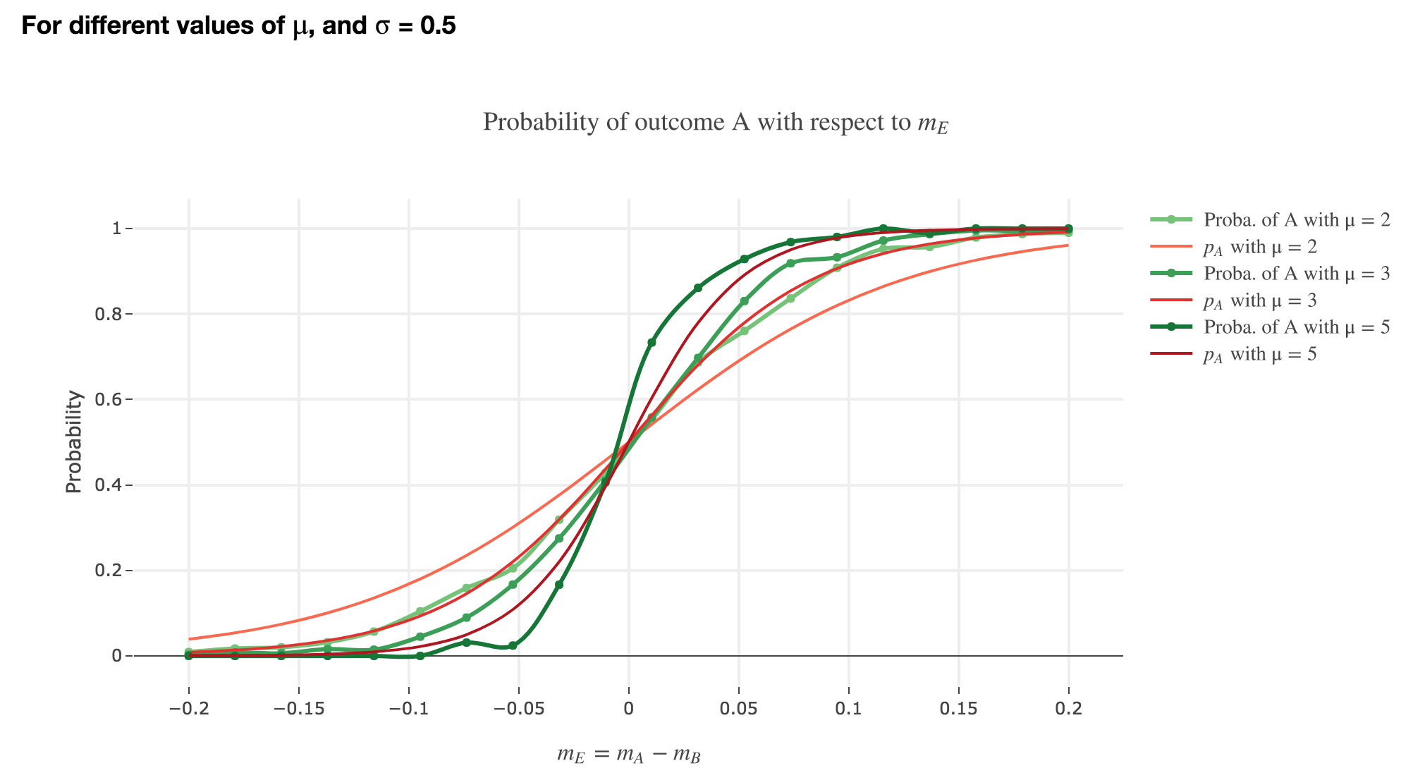
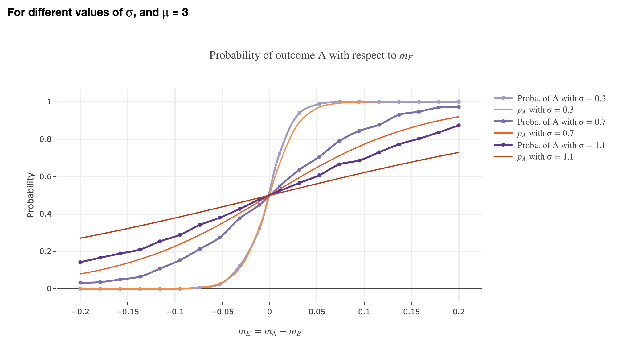
We see that the empirical probability of outcome $A$ matches more and more $p_A$ (when it comes to the shape of the curve):
-
as $μ$ increases
-
as $σ$ decreases (with an almost perfect match above for $σ = 0.3$)
Leave a comment