Lecture 4: Drift-diffusion models
Reminder: differential equations we’ll encounter
\[\frac{d f}{dt}(t) = A(f(t), t)\]NB: Beware of the units: Ex:
\[\dot{x} = α - x\]is not homogenous, $\dot{x}$ has the unit of $x$ divided by time.
Numerically solving differential equations
\[\frac{d f}{dt}(t) = A(f(t), t)\]Time-discretize it:
\[\frac{Δ f}{Δ t}(t) = A(f(t), t) \\ ⟺ \frac{f(t+Δt) - f(t)}{Δt}(t) = A(f(t), t) \\ ⟺ f(t+Δt) = f(t) + Δt A(f(t), t)\]Stochastic differential equations
Far more difficult: methods to solve them have been designed in late 20th century.
We’ll content ourselves with simulating them
White noise
Noise with all the frequencies (as if we added an infinite amount of sine funtions, ranging over an infinite amount of frequencies).
\[\underbrace{⟨ξ(t) \cdot ξ(t+τ)⟩}_{\text{expected value}} = δ(τ)\]- Delta-function (Dirac function):
-
intuitively: zero everwhere except at $t = 0$, where it “diverges to $+∞$”
NB:
-
Expected value: $⟨ξ(t)⟩ = 0$
-
Variance: infinite (you sum all the frequencies)
Differential equation with white noise
\[\frac{Δ f}{Δ t}(t) = A(f(t), t) + α ξ(t)\]After discretizing:
\[f(t+Δt) = f(t) + Δt A(f(t), t) + α \, \underbrace{Δt \, ξ(t)}_{≝ \, W(t) \; \text{(Wiener process)}}\]where $Var(W(t)) = Δt$
It comes from Ito calculus. Basic idea of Brownian motion.
So overall:
\[f(t+Δt) = f(t) + Δt A(f(t), t) + α \, \sqrt{Δt} \; η(t)\]where $η(t)$ is coming from a Gaussian process $\sim 𝒩(0, 1)$: at each time-step, you draw $η(t)$ from a Gaussian distribution $\sim 𝒩(0, 1)$.
NB: So be careful when intergrating: if you use a package when solving stochastic differential equations, it might not work! Do it by hand.
Model of behavior: neural implementation
What are neurons actually computing in the brain?
Behavior, cognition ⟹ Neural implementation
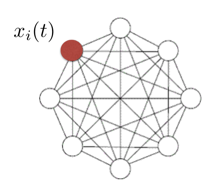
Hopfield Network
(short paper: 4 pages long, cited thousands of times)
- Associative memory:
-
when you have a hint/stimulus, you can retrieve the memory associated with it
Idea:
-
memories = fixed points of the dynamics
- i.e in the graph of neurons, each node is associated with a function $x_i(t)$. A fixed point is such a function which stays constant when its envionment/neighbors are fixed.
-
large networks can store
-
initial conditions = hints for memory retrieval
Decision making
Huge field related to many areas: neuroscience, economy, psychology, …
Perceptual decision making: an animal has to make a choice when presented a certain stimulus
The animal is forced to say something about the stimulus (ex: which one larger, brighter, etc…).
Ex: Experience with monkeys:
there is a bunch of dots presented to the animal: the animal is rewarded if it guesses which side (right or left) has had the most dots (eye-tracking system to see where the animal is staring).
In the visual area MT (called V5), neurons seem to respond to motion direction.
As you increase the coherence of the motion, the firing distribution of these neurons are more and more distinguished.
Control experiment: by perturbing activity in MT, behavior is perturbed.
Now: how does the brain process information from MT?
The area LIP is very important in doing so.
- The lower the coherence, the larger the reaction time.
- There is a threshold mechanism: the neurons accumulate information a certain amount of information before making a decision
- This decision is correlated to a firing rate threshold in the LIP area
There are 2 completely different models which both have noise and a threshold mechanism to describe this in computational neuroscience literature.
Wang’s model (2002)
You have different competing populations of neurons:
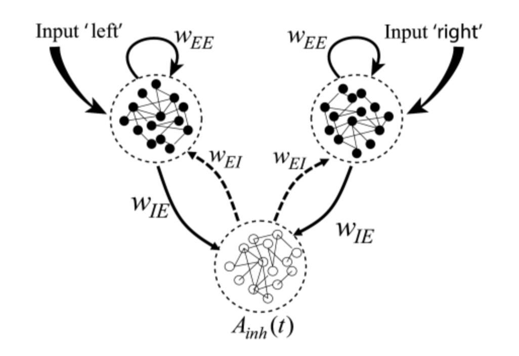
- a population for “right”
- a population for “left”
- an inhibiting population
⇒ called the winner take all mechanism
Drift-diffusion model (Ratcliff and Rouder, 1998)
-
more theoretical: originally theoretical, didn’t model neurons per se at first
-
but can be applied to model the behavior of LIP neurons
There’s a decision variable $x$, which represent the firing rate of LIP neurons
\[x(t_0) = x_0\\ \frac{dx}{dt} = (I_A - I_B) + σ ξ(t)\]where
- $ξ(t)$ is a white noise
- $I_A - I_B$ is a “drift force” for A (left) and B (right) in MT
and there are thresholds (positive and negative) above (or under) which the decision is made:
\[\text{Thresholds: } 𝛩_A, 𝛩_B\]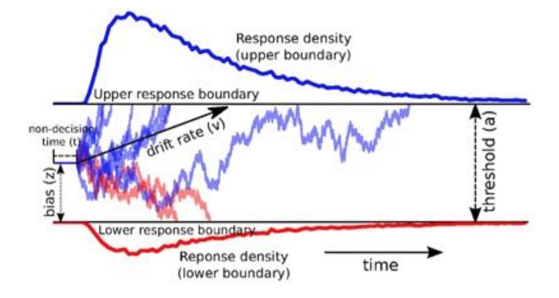
Reaction time:
\[t_A = \min \lbrace t \mid x(t) = 𝛩_A \rbrace\\ t_B = \min \lbrace t \mid x(t) = 𝛩_B \rbrace\]
Leave a comment