Tutorial 1: Reinforcement Learning
Tutorial 1: Reinforcement Learning
Kexin Ren & Younesse Kaddar (Lecturer: Nicolas Perrin)
1. Markov Decision Problems
Our problem is a Markov Decision Problems (MDP) which is described by a tuple $(𝒳, 𝒰, 𝒫_0, 𝒫,r,γ)$ where $𝒳$ is the state-space, $𝒰$ the action-space, $𝒫_0$ the distribution of the initial state, $𝒫$ the transition function, $r$ the reward function, and $γ ∈ [0, 1]$ a parameter called the discount factor.
The state in which the robot starts, denoted $x_0$, is drawn from the initial state distribution $𝒫_0$. We will choose it such that the robot always starts in state $0$. Then, given the state $x_t$ at time $t$ and the action $u_t$ at that same time, the next state $x_{t+1}$ depends only on $x_t$ and $u_t$ according to the transition function $𝒫$:
\[𝒫(x_t, u_t, x_{t+1}) = {\rm P}(x_{t+1} \mid x_t, u_t)\]If the robot tries to get out of the grid (for example if it uses action $N$ in state $0$), it will stay in his current state. The robot also receives a reward $r_t$ according to the reward function $r(x_t, u_t)$, which depends on the state $x_t$ and the action $u_t$. We choose to give a reward $1$ when the robot is in state $15$ and does the action $NoOp$, and $0$ for any other state-action pair.
Questions
1. Define self.gamma
We may set $γ$ to be equal to $0.95 ∈ [0, 1]$, for instance.
class mdp():
    def __init__(self):
        # [...]
        self.gamma = 0.95
2. In __init__(self), define P0, the distribution of the initial state.
As the robot always starts in state $0$: $𝒫_0$ is equal to the Dirac measure $δ_0$
class mdp():
    def __init__(self):
        # [...]

        self.P0 = np.zeros(self.nX)
        self.P0[0] = 1

        # [...]
3. Write down the transition probabilities for each triplet $𝒫(\text{state}, \text{action}, \text{next state})$ for the example above
class mdp():
    def __init__(self):
        # [...]

        self.P = np.empty((self.nX,self.nU,self.nX))
        self.P[:,N,:]=  np.array([
            [1.0, 0.0, 0.0, 0.0, 0.0, 0.0, 0.0, 0.0, 0.0, 0.0, 0.0, 0.0, 0.0, 0.0, 0.0, 0.0],
            [1.0, 0.0, 0.0, 0.0, 0.0, 0.0, 0.0, 0.0, 0.0, 0.0, 0.0, 0.0, 0.0, 0.0, 0.0, 0.0],
            [0.0, 1.0, 0.0, 0.0, 0.0, 0.0, 0.0, 0.0, 0.0, 0.0, 0.0, 0.0, 0.0, 0.0, 0.0, 0.0],
            [0.0, 0.0, 1.0, 0.0, 0.0, 0.0, 0.0, 0.0, 0.0, 0.0, 0.0, 0.0, 0.0, 0.0, 0.0, 0.0],
            [0.0, 0.0, 0.0, 0.0, 1.0, 0.0, 0.0, 0.0, 0.0, 0.0, 0.0, 0.0, 0.0, 0.0, 0.0, 0.0],
            [0.0, 0.0, 0.0, 0.0, 1.0, 0.0, 0.0, 0.0, 0.0, 0.0, 0.0, 0.0, 0.0, 0.0, 0.0, 0.0],
            [0.0, 0.0, 0.0, 0.0, 0.0, 1.0, 0.0, 0.0, 0.0, 0.0, 0.0, 0.0, 0.0, 0.0, 0.0, 0.0],
            [0.0, 0.0, 0.0, 0.0, 0.0, 0.0, 1.0, 0.0, 0.0, 0.0, 0.0, 0.0, 0.0, 0.0, 0.0, 0.0],
            [0.0, 0.0, 0.0, 0.0, 0.0, 0.0, 0.0, 0.0, 1.0, 0.0, 0.0, 0.0, 0.0, 0.0, 0.0, 0.0],
            [0.0, 0.0, 0.0, 0.0, 0.0, 0.0, 0.0, 0.0, 1.0, 0.0, 0.0, 0.0, 0.0, 0.0, 0.0, 0.0],
            [0.0, 0.0, 0.0, 0.0, 0.0, 0.0, 0.0, 0.0, 0.0, 1.0, 0.0, 0.0, 0.0, 0.0, 0.0, 0.0],
            [0.0, 0.0, 0.0, 0.0, 0.0, 0.0, 0.0, 0.0, 0.0, 0.0, 1.0, 0.0, 0.0, 0.0, 0.0, 0.0],
            [0.0, 0.0, 0.0, 0.0, 0.0, 0.0, 0.0, 0.0, 0.0, 0.0, 0.0, 0.0, 1.0, 0.0, 0.0, 0.0],
            [0.0, 0.0, 0.0, 0.0, 0.0, 0.0, 0.0, 0.0, 0.0, 0.0, 0.0, 0.0, 1.0, 0.0, 0.0, 0.0],
            [0.0, 0.0, 0.0, 0.0, 0.0, 0.0, 0.0, 0.0, 0.0, 0.0, 0.0, 0.0, 0.0, 1.0, 0.0, 0.0],
            [0.0, 0.0, 0.0, 0.0, 0.0, 0.0, 0.0, 0.0, 0.0, 0.0, 0.0, 0.0, 0.0, 0.0, 1.0, 0.0]])

        self.P[:,S,:] =  self.P[::-1,N,::-1]

        self.P[:,E,:] = np.array([
            [0.0, 0.0, 0.0, 0.0, 1.0, 0.0, 0.0, 0.0, 0.0, 0.0, 0.0, 0.0, 0.0, 0.0, 0.0, 0.0],
            [0.0, 0.0, 0.0, 0.0, 0.0, 1.0, 0.0, 0.0, 0.0, 0.0, 0.0, 0.0, 0.0, 0.0, 0.0, 0.0],
            [0.0, 0.0, 0.0, 0.0, 0.0, 0.0, 1.0, 0.0, 0.0, 0.0, 0.0, 0.0, 0.0, 0.0, 0.0, 0.0],
            [0.0, 0.0, 0.0, 0.0, 0.0, 0.0, 0.0, 1.0, 0.0, 0.0, 0.0, 0.0, 0.0, 0.0, 0.0, 0.0],
            [0.0, 0.0, 0.0, 0.0, 0.0, 0.0, 0.0, 0.0, 1.0, 0.0, 0.0, 0.0, 0.0, 0.0, 0.0, 0.0],
            [0.0, 0.0, 0.0, 0.0, 0.0, 0.0, 0.0, 0.0, 0.0, 1.0, 0.0, 0.0, 0.0, 0.0, 0.0, 0.0],
            [0.0, 0.0, 0.0, 0.0, 0.0, 0.0, 0.0, 0.0, 0.0, 0.0, 1.0, 0.0, 0.0, 0.0, 0.0, 0.0],
            [0.0, 0.0, 0.0, 0.0, 0.0, 0.0, 0.0, 0.0, 0.0, 0.0, 0.0, 1.0, 0.0, 0.0, 0.0, 0.0],
            [0.0, 0.0, 0.0, 0.0, 0.0, 0.0, 0.0, 0.0, 0.0, 0.0, 0.0, 0.0, 1.0, 0.0, 0.0, 0.0],
            [0.0, 0.0, 0.0, 0.0, 0.0, 0.0, 0.0, 0.0, 0.0, 0.0, 0.0, 0.0, 0.0, 1.0, 0.0, 0.0],
            [0.0, 0.0, 0.0, 0.0, 0.0, 0.0, 0.0, 0.0, 0.0, 0.0, 0.0, 0.0, 0.0, 0.0, 1.0, 0.0],
            [0.0, 0.0, 0.0, 0.0, 0.0, 0.0, 0.0, 0.0, 0.0, 0.0, 0.0, 0.0, 0.0, 0.0, 0.0, 1.0],
            [0.0, 0.0, 0.0, 0.0, 0.0, 0.0, 0.0, 0.0, 0.0, 0.0, 0.0, 0.0, 1.0, 0.0, 0.0, 0.0],
            [0.0, 0.0, 0.0, 0.0, 0.0, 0.0, 0.0, 0.0, 0.0, 0.0, 0.0, 0.0, 0.0, 1.0, 0.0, 0.0],
            [0.0, 0.0, 0.0, 0.0, 0.0, 0.0, 0.0, 0.0, 0.0, 0.0, 0.0, 0.0, 0.0, 0.0, 1.0, 0.0],
            [0.0, 0.0, 0.0, 0.0, 0.0, 0.0, 0.0, 0.0, 0.0, 0.0, 0.0, 0.0, 0.0, 0.0, 0.0, 1.0]])

        self.P[:,W,:] = self.P[::-1,E,::-1]

        self.P[:,NoOp,:]=  np.eye(self.nX)

        # [...]
4. Define the reward function r, stored in the matrix self.r
As reward is equal to $1$ if the robot is in state $15$ and does the action $NoOp$, and $0$ otherwise:
class mdp():
    def __init__(self):
        # [...]
        self.r = np.zeros((self.nX, self.nU))
        self.r[15, NoOp] = 1
2. Dynamic Programming
The overall goal is to maximize
\[𝔼\left[ \sum\limits_{ t=0 }^∞ γ^t r(x_t, u_t) \mid x_0 \sim 𝒫_0, \; x_{t+1} \sim 𝒫(x_t, u_t, \bullet) \right]\]A policy is a mapping $π : X ⟶ U$ that assigns, to each state $x$, an action $u ≝ π(x)$ that the robot should execute whenever in state $x$.
The state value of a policy $π$ is the total discounted reward that the robot expects to receive when starting from a given state $x$ and following policy $π$:
\[V^π(x) ≝ 𝔼\left[ \sum\limits_{ t=0 }^∞ γ^t r(x_t, u_t) \mid x_0 = x, \; u_t = π(x_t), \; x_{t+1} \sim 𝒫(x_t, u_t, \bullet) \right]\]The state-action value of a policy $π$ is the total discounted reward that the robot expects to receive when starting from a given state $x$, taking the action $u$ and then following policy $π$:
\[Q^π(x, u) ≝ 𝔼\left[ \sum\limits_{ t=0 }^∞ γ^t r(x_t, u_t) \mid x_0 = x, \; u_0 = u, \, u_t = π(x_t), \; x_{t+1} \sim 𝒫(x_t, u_t, \bullet) \right]\]The optimal policy is the policy $π^\ast$ such that for every state:
\[∀x ∈ 𝒳, ∀ π ∈ 𝒰^𝒳, \; V^\ast(x) ≥ V^π(x)\]In particular, we have:
\[\begin{cases} V^\ast(x) = \max_u Q^\ast(x, u) \\ π^\ast(x) = {\rm argmax}_u Q^\ast(x, u) \qquad (3)\\ \end{cases}\]2.1 Value Iteration
It stems from the above that:
\[Q^\ast = r(x, u) + γ \sum\limits_{ y ∈ 𝒳 } 𝒫(x, u, y) \underbrace{V^\ast(y)}_{= \, \max_u Q^\ast(x, u)} \qquad ⊛\]out of which we get a recursive algorithm to compute $Q^\ast$:
\[Q^{(k+1)} = r(x, u) + γ \sum\limits_{ y ∈ 𝒳 } 𝒫(x, u, y) \, \max_u Q^{(k)}(x, u) \qquad (8)\]1. Set the proper ranges in the for i and for j loops.
iranges over the statesjranges over the actions
therefore:
def VI(self):
    Q = np.zeros((self.nX,self.nU))
    # [...]

        for i in range(self.nX):
            for j in range(self.nU):
                # [...]
2. Complete the assignment Q[i,j] =
Based on the equation $(8)$:
Q[i,j] = self.r[i,j] + self.gamma * np.sum(self.P[i,j,:] * Qmax)
As a result, the VI method becomes:
def VI(self):
    Q = np.zeros((self.nX, self.nU))
    pol = N*np.ones((self.nX, 1))
    quitt = False
    iterr = 0

    while quitt==False:
        iterr += 1
        Qold = Q.copy()
        Qmax = Qold.max(axis=1)

        for i in range(self.nX):
            for j in range(self.nU):
                Q[i,j] = self.r[i,j] + self.gamma * np.sum(self.P[i,j,:] * Qmax)

        Qmax = Q.max(axis=1)
        pol =  np.argmax(Q,axis=1)
        if (np.linalg.norm(Q-Qold))==0:
            quitt = True
    return [Q,pol]
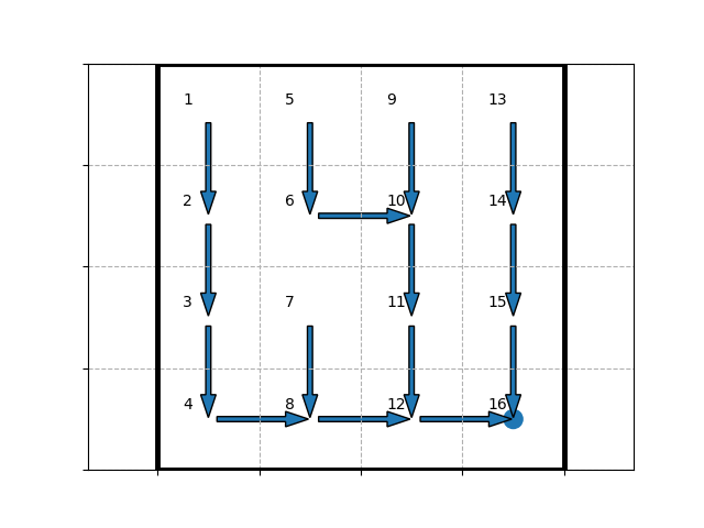
and by running python run.py, the following policy figure is displayed:
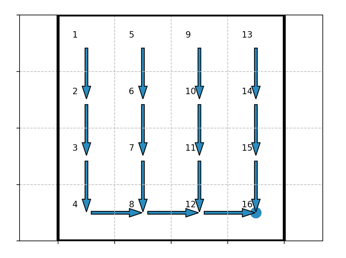
which makes sense, since the state $15$ (denoted by $16$ on the figure) is the most attractive with its reward of $1$ (whereas the other states have a zero reward).
3. Add a second goal: modify the reward function to give $0.9$ when the robot is in state $5$ and does not move. Explain when and why the robot chooses to go to this new goal instead of the first one. Explain what parameter is responsible of this behaviour.
The discount factor $γ$ determines a tradeoff between exploration (exploring farther states) and exploitation/greediness (exploiting the rewards of the nearby one). As it happens: the smaller the parameter $γ$, the more the robot tends to exploit the closest state associated with a (strictly) positive reward (even if there might be a state farther on which a given action leads to a bigger reward).
Here, there are two different optimal policies, depending on the value of $γ$:
| Value of $γ$ | Optimal Policy |
|---|---|
| Greedier policy: $γ < γ_0 ≝ \sqrt{0.9}$ | 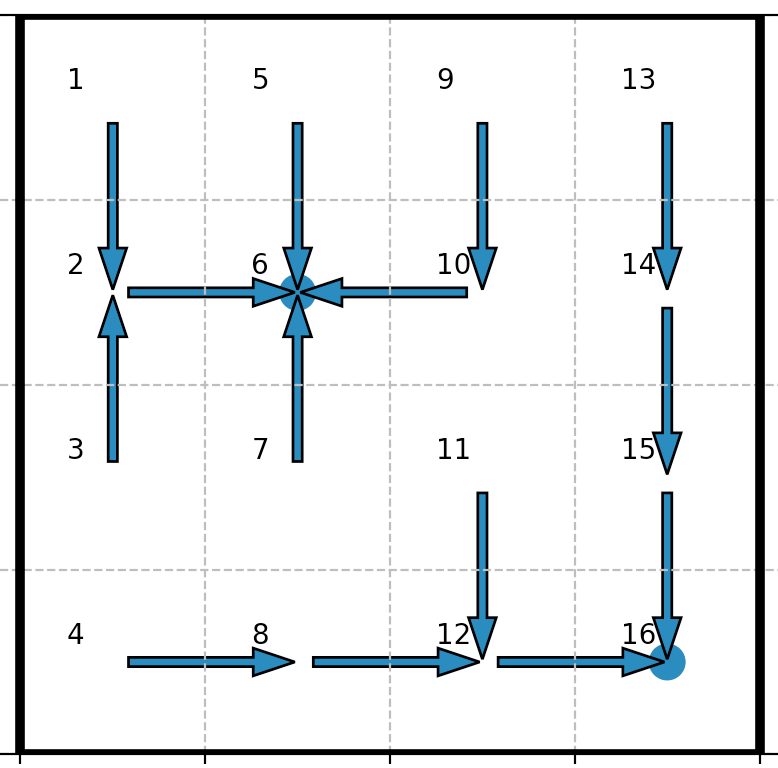 |
| More exploratory policy: $γ ≥ γ_0$ | 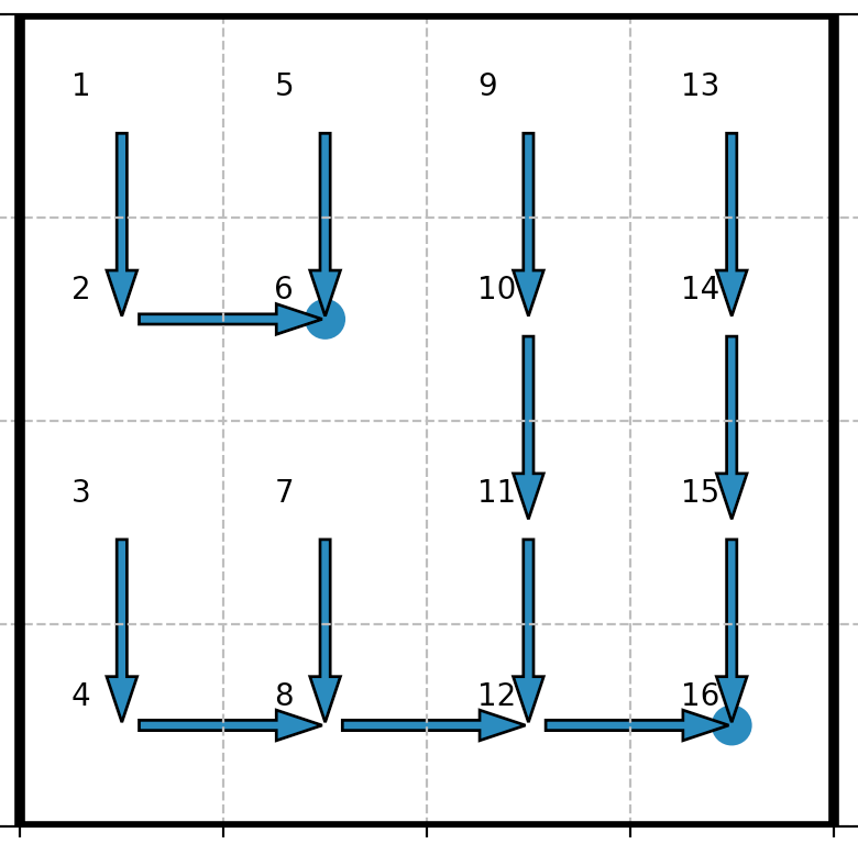 |
When it comes to the greedier policy: for states close to the state $5$ (denoted by $6$ on the pictures), the robot tends to head to the state $5$, even if its reward ($=0.9$) is inferior the reward ($=1$) of the state $15$ (denoted by $16$ on the pictures)
On the contrary, with the more exploratory policy: apart from the states $0, 1$ and $4$ (which are one step away from the state $5$), the robot favors the state $15$, i.e. the long-term bigger reward over the smaller yet closer (for the states $2, 6, 8$ and $9$) reward of the state $5$.
4. Change self.P to implement stochastic (non-deterministic) transitions. Use comments in the code to describe the transitions you chose and the results you observed while running VI on the new transitions you defined.
NB: in this question, for convenience
- we’ll call a state out of which the transition function is non-deterministic a stochastic state
- we’ll use the old reward function, which amounts to zero everywhere except on state $15$ when the robot doesn’t move (in which case it is set to be $1$)
To implement stochastic transitions, we use the first state and the seventh state as examples, with the following code (having non-deterministic transitions for every state overcomplicate things: one state with non-deterministic transitions is enough to have a good idea of what’s going on):
pos = np.random.rand(5)
n = 0 # n = 0 for 1st state, n = 6 for 7th state
for i in range(self.nU):
	self.P[n,i,np.where(self.P[n,i,:]==1)]=pos[i]/sum(pos)
We found that, when the first step (at state $0$) is stochastic, the result is the same as the deterministic one (as shown in Figure 2.1.4.1) which makes sense because all routes will actually weigh the same under these conditions; when the 7th state (state $6$) is stochastic, no neighboring state of state $6$ will have the agent (via the optimal policy) choose to go through state $6$ (as shown in Figure 2.1.4.2), because there is a possibility of going “backwards” (i.e. not towards to the most attractive state (due to its reward), state $15$) on state $6$, which will reduce the $Q$-value of other states heading for state $6$.
NB: in the figures, the states range from $1$ to $16$
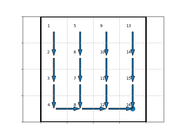
On the whole, with a stochastic transition function: the less “stable” (i.e. likely to lead to a given state for a given action) a stochastic state is, the more it is likely to be averted, if it is on the way to a high-reward state.
2.2. Policy Iteration
By definition of the state value function of a given policy $π$, we have:
\[V^π(x) = r(x, π(x)) + γ \sum\limits_{ y ∈ 𝒳 } 𝒫(x, π(x), y) V^π(y) \qquad ⊛⊛\]But as $𝒳$ is finite: by setting $\textbf{V}_π$ (resp. $\textbf{R}_π$) to be the vector-matrix $(V^π(x))_{x ∈ 𝒳}$ (resp. $(r(x, π(x)))_{x ∈ 𝒳}$), and
\[\textbf{P}_π ≝ (𝒫(x, π(x), y))_{\substack{x ∈ 𝒳 \\ y ∈ 𝒳}}\]it comes that
\[\begin{align*} & \; \textbf{V}_π = \textbf{R}_π + γ \textbf{P}_π \textbf{V}_π\\ ⟺ & \; \textbf{V}_π =(\textbf{I} - γ \textbf{P}_π)^{-1} \textbf{R}_π && (9)\\ \end{align*}\]which yields another algorithm to compute the optimal policy, along with
\[\begin{cases} Q^π(x, u) = r(x, u) + γ \sum\limits_{ y ∈ 𝒳 } 𝒫(x, u, y) V^π(y) && (6)\\ π^{(k+1)}(x) = {\rm argmax}_u {Q^π}^{(k)}(x, u) && (10)\\ \end{cases}\]1. Fill the code PI(self) to implement policy iteration, and test it. Compare the converge speed of VI and PI.
Using the previous equations, it comes that:
def PI(self):
    Q = np.empty((self.nX, self.nU))
    pol = N*np.ones(self.nX, dtype=np.int16)
    R = np.zeros(self.nX)
    P = np.zeros((self.nX, self.nX))
    quitt = False
    iterr = 0

    while quitt==False:
        iterr += 1

        for i in range(self.nX):
            R[i] = self.r[i,pol[i]]
            for j in range(self.nX):
                P[i,j] = self.P[i,pol[i],j]

        V = np.dot(np.linalg.inv(I-self.gamma*P), R)

        for i in range(self.nX):
            for j in range(self.nU):
                Q[i,j] = self.r[i,j] + self.gamma * np.sum(self.P[i,j,:] * V)
                print(Q[i,j])

        pol_old = pol.copy()
        pol = np.argmax(Q, axis=1)

        if np.array_equal(pol, pol_old):
            quitt = True

    return [Q, pol]
We compared the convergences of VI and PI and found that, VI algorithm converges after 667 iterations while the PI algorithm converges after 3 iterations, supporting the fact that PI is more efficient than VI (gamma is set to 0.95).
In a terminal:
python -mtimeit -s'import mdp' 'mdp.mdp().PI()'
>> 100 loops, best of 3: 2.66 msec per loop

python -mtimeit -s'import mdp' 'mdp.mdp().VI()'
>> 10 loops, best of 3: 250 msec per loop
which suggests that
PIis approximately 100 times faster thanVI
3. Reinforcement Learning: Model-free approaches
3.1. Temporal Difference Learning (TD-learning)
Based on $⊛$ and $⊛⊛$, we get:
\[\begin{cases} V^π(x) = 𝔼\left[r(x, π(x)) + γ V^π(y) \mid y \sim 𝒫(x, π(x), \bullet)\right] &&(11)\\ Q^\ast(x, u) = 𝔼\left[r(x, u) + γ \max_v Q^\ast(y, v) \mid y \sim 𝒫(x, u, \bullet)\right] &&(12)\\ \end{cases}\]as a result of which we define the temporal difference errors (TD errors):
\[\begin{cases} δ_{V^π}(x) ≝ 𝔼\left[r(x, π(x)) + γ V^π(y) - V^π(x) \mid y \sim 𝒫(x, π(x), \bullet)\right] &&(13)\\ δ_{Q^\ast}(x, u) ≝ 𝔼\left[r(x, u) + γ \max_v Q^\ast(y, v) - Q^\ast(x, u) \mid y \sim 𝒫(x, u, \bullet)\right] &&(14)\\ \end{cases}\]3.2. TD(0)
At time $t$, we denote by
- $V^{(t})$ the estimation of the state value function
- $x_t$ the current state
- $δ_t ≝ δ_{V^{(t)}}(x_t)$
- $α$ the learning rate
From the $δ$-rule, the following update of the state value function can be derived:
\[V^{(t+1)}(x_t) = V^{(t)}(x_t) + α \underbrace{δ_t}_{\rlap{≝ \; r(x_t, u_t) + γ V^{(t)}(x_{t+1}) - V^{(t)}(x_t)}} \quad\qquad (15)\]1. Open the file mdp.py, and implement a function called MDPStep. This function returns a next state and a reward given a state and an action. Hint: To draw a number according to a vector of probabilities, you can use the function discreteProb.
def MDPStep(self,x,u):
    # This function executes a step on the MDP M given current state x and action u.
    # It returns a next state y and a reward r
    y = self.discreteProb(self.P[x,u,:]) # y is sampled according to the distribution self.P[x,u,:]
    r = self.r[x,u] # r is be the reward of the transition
    return [y,r]
2. Fill-in the missing lines in the TD function, which implements $TD(0)$. To obtain samples from MDP, you will use the MDPStep function
def TD(self,pol):
    V = np.zeros((self.nX,1))
    nbIter = 100000
    alpha = 0.1
    for i in range(nbIter):
        x = np.floor(self.nX*np.random.random()).astype(int)
        [y, r] = self.MDPStep(x, pol[x])
        V[x] += alpha * (r + self.gamma * V[y] - V[x])
    return V
By
-
modifying
run.pyso that one computes:[Q,pol] = m.PI() V = m.TD(pol) -
and adding the line
print(np.argsort(V,axis=0))in the
TDmethod, just before the return, to sort the states according to their estimated value (in increasing order)
it appears that the estimated values are sorted as follows:
\[\begin{align*} \quad & V^π(1) \;\, ≤ V^π(3) \;\, ≤ V^π(9) \;\, ≤ \;\, V^π(4)\\ ≤ \; & V^π(13) ≤ V^π(2) \;\, ≤ V^π(5) \;\, ≤ V^π(7)\\ ≤ \; & V^π(10) ≤ V^π(8) \;\, ≤ V^π(11) ≤ V^π(14)\\ ≤ \; & V^π(6) \;\, ≤ V^π(12) ≤ V^π(15) ≤ V^π(16) \end{align*}\]for
-
the deterministic transition function and the reward function of question 2.1.3. (the reward is null everywhere except at state $5$ (where it amounts to $0.9$) and state $15$ (where it amounts to $1$) when the robot doesn’t move)
-
the following policy ($γ < \sqrt{0.9}$):

which makes perfect sense, intuitively.
3. Write a function compare that takes in input a state value function $V$, a policy $π$, a state-action value function $Q$, and returns True if and only if $V$ and $Q$ are consistent with respect to $π$ up to some precision, i.e. if $∀x ∈ 𝒳, V^π(x) = Q^π(x, π(x)) ± ε$.
We are asked to program a function which test if $∀x ∈ 𝒳, \vert V^π(x) - Q^π(x, π(x)) \vert ≤ ε_{max}$, for a threshold value $ε_{max}$: i.e. if the infinity norm of the difference of the vectors is smaller than $ε_{max}$.
def compare(self,V,Q,pol,eps=0.0001):
    Q_pol = np.array([[Q[x, pol[x]]] for x in range(V.size)])
    return np.linalg.norm(V-Q_pol, ord=np.inf)<eps
4. Use the compare function to verify that $TD(0)$ converges towards the proper value function, using it on the policy returned by VI or PI.
[Q1,pol1] = m.VI()
[Q2,pol2] = m.PI()

V1 = m.TD(pol1)
V2 = m.TD(pol2)

print(m.compare(V1,Q1,pol1))
print(m.compare(V2,Q2,pol2))
yields True and True, so $TD(0)$ does converge towards the proper value function.
3.3. Q-Learning
In accordance with the softmax-policy:
\[π^{(t)}(u \mid x) ≝ \frac{\exp(Q^{(t)}(x, u)/τ)}{\sum\limits_{ v ∈ 𝒰 } \exp(Q^{(t)}(x, v)/τ)}\]we update the state-action value function as follows:
\[Q^{(t+1)}(x_t, u_t) = Q^{(t)}(x_t, u_t) + α \left[r(x_t, u_t) + γ \max_{u_{t+1} ∈ 𝒰} Q^{(t)}(x_{t+1}, u_{t+1}) - Q^{(t)}(x_t, u_t)\right] \qquad (16)\]1. Implement the function softmax that returns the soft-max policy.
def softmax(self,Q,x,tau):
    # Returns a soft-max probability distribution over actions
    # Inputs :
    # - Q : a Q-function reprensented as a nX times nU matrix
    # - x : the state for which we want the soft-max distribution
    # - tau : temperature parameter of the soft-max distribution
    # Output :
    # - p : probabilty of each action according to the soft-max distribution
    # (column vector of length nU)

    p = np.exp(Q[x,:]/tau)
    return p/np.sum(p)
2. Fill-in the missing lines to implement the QLearning function.
def QLearning(self,tau):
    # This function computes the optimal state-value function and the corresponding policy using Q-Learning

    # Initialize the state-action value function
    Q = np.zeros((self.nX,self.nU))

    # Run learning cycle
    nbIter = 100000
    alpha = 0.01
    for i in range(nbIter):
        # Draw a random state
        x = np.floor(self.nX*np.random.random()).astype(int)

        # Draw an action using a soft-max policy
        u = self.discreteProb(self.softmax(Q,x,tau))

        # Perform a step of the MDP
        [y,r] = self.MDPStep(x, u)

        # Update the state-action value function with Q-Learning
        Q[x,u] += alpha * (r + self.gamma * np.max(Q[y,:]) - Q[x,u])

    # Compute the corresponding policy
    Qmax = Q.max(axis=1)
    pol =  np.argmax(Q,axis=1)
    return [Qmax,pol]
3. Run $Q$-Learning several times. What do you observe?
NB: in this question, the numbering of the states is the displayed one by plotPolicy (i.e. the states range from $1$ to $16$).
We found that the policy is stochastic, except that for the rightmost column (i.e. states $13, 14$ and $15$), bottom row (i.e. states $4, 8, 12$) and of course, state $16$, the policy is fixed. The states in the rightmost column always lead to the South action, towards the state $16$, while the states in the bottom row always lead to the East action, towards the state $16$.
This makes sense because for the rightmost column and the bottom row, there is only one choice of action (or direction) for them which will go towards the state $16$, and the robot will learn the only right direction when soft-max is applied. Unlike states in these two lines, other states have actions associated to them in a non-deterministic way, as a stochastic strategy is used in the algorithm.
4. Compare the state-value function and the policy computed using $Q$-Learning with the ones you obtained with VI and PI.
NB: in this question, for convenience, the old reward function is referred to (which amounts to zero everywhere except on state $16$ when the robot doesn’t move (in which case it is set to be $1$))
Regarding the policy:
-
on the one hand,
VIandPIare deterministic algorithms, always ouputting the optimal (up to the precision ofnp.linalg.norm(Q-Qold) == 0andnp.array_equal(pol, pol_old)) policy: we exploration/exploitation tradeoff is dealt with by the discount factor $γ$ -
on the other hand, $Q$-Learning generates a policy (converging to the optimal one as
nbIterincreases) non-deterministically: on top of the discount factor $γ$, there is another layer which has an impact on the exploration/exploitation tradoff: the softmax policy used to draw the very samples that enable us to update the $Q$-function
Regarding the state-value function:
-
the results may differ for every trial of $Q$-Learning depending on the stochastic experience of the robot, while the results remain the same each time for
VIandPI(which are deterministic). -
moreover, the state-value matrices of
VIandPIhave coefficients that don’t vary “too much”: they range over smaller values (usually $13$ - $20$), and the actions towards the high-reward state $16$ lead to a higher value, as expected. On the contrary, the state-value matix of $Q$-Learning usually presents (with respect to its coefficients) more discrepancies: with disparity in value magnitude and sometimes no apparent correlation between the value and direction towards the high-reward state $16$.
4. Model-Based Reinforcement Learning (MBRL)
Real-Time Dynamic Programming:
We update the estimate of the transition probabilty $\hat{𝒫}^{(t)}$ as follows:
\[\hat{𝒫}^{(t)}(x_t, u_t, y) ≝ \left(1 - \frac 1 {N_t(x_t, u_t)}\right) \hat{𝒫}^{(t)}(x_t, u_t, y) + \frac 1 {N_t(x_t, u_t)} \mathbb{1}_{y = x_{t+1}} \qquad (17)\]where $N_t(x,u)$ is the number of visits to the pair $(x,u)$ before (and including) time $t$.
As for the reward function estimate:
\[\hat{r}^{(t+1)}(x_t, u_t) ≝ r_t \qquad (18)\]Those are used in the following updating rule:
\[Q^{(t+1)}(x_t, u_t) ≝ \hat{r}^{(t+1)}(x_t, u_t) + γ \sum\limits_{ y ∈ 𝒳 } \hat{𝒫}^{(t+1)}(x_t, u_t, y) \max_{v ∈ 𝒰} Q^{(t)}(y, v) \qquad (19)\]1. Fill-in RTDP (Real-Time Dynamic Programming) function
def RTDP(self):
    Q = np.zeros((self.nX,self.nU))
    hatP = np.ones((self.nX,self.nU,self.nX))/self.nX
    N = np.ones((self.nX,self.nU))

    nbIter = 10000

    for iterr in range(nbIter):
        # Draw a random pair of state and action
        x = np.floor(self.nX*np.random.random()).astype(int)
        u = np.floor(self.nU*np.random.random()).astype(int)

        # One step of the MDP for this state-action pair
        [y,r] = self.MDPStep(x,u)

        # Compute the estimate of the transition probabilities
        hatP[x,u,:] *= (1 - 1/N[x, u])
        hatP[x,u,:] += (np.arange(self.nX) == y).astype(int)/N[x, u]

        # Updating rule for the state-action value function
        Qmax = Q.max(axis=1)
        Q[x,u] = r + self.gamma * np.sum(hatP[x,u,:]*Qmax)

        N[x,u] += 1

    Qmax = Q.max(axis=1)
    pol =  np.argmax(Q,axis=1)

    return [Qmax,pol]
2. Suppose now that the reward is stochastic: modify MDPStep by adding a Gaussian noise of standard deviation $0.1$ to the reward. What happens if you set the standard deviation to $1.0$?
def MDPStep(self,x,u,sigma=0.1):
    # This function executes a step on the MDP M given current state x and action u.
    # It returns a next state y and a reward r
    y = self.discreteProb(self.P[x,u,:]) # y is sampled according to the distribution self.P[x,u,:]
    r = self.r[x,u] + sigma * np.random.randn() # r is be the reward of the transition
    return [y,r]
Noisy rewards have an effect on how good a job the computed policy is doing at maximizing the overall cumulated rewards (we may call that the efficiency of the policy). The smaller the standard deviation of the noise, the more efficient the computed policy becomes, since the rewards that were encountered during RTDP tend to be closer and closer to their regular/actual values. It all hinges on how the standard deviation of the noise compares to the order of magnitude of the mean rewards.
With a small (compared to how large the mean rewards can get) noise standard deviation (e.g. $0.1 < 1 = \text{reward of state } 16$), the policy becomes just a little less efficient. However, with a big noise standard deviation value (e.g. $1$, which is as large as the mean rewards can get), the robot is completely confused: for instance, it is difficult to draw any conclusion when receiving a reward of $1$ on a given sample: it may mean that the current state-action pair has
- a mean reward of $0$ (non-attractive state) with a noise of $+1$
- or a mean reward of $1$ (highly attractive state) with a noise of $0$
As a result, one can barely figure out any reliable solution.


3. Implement RTDP2, a variant of RTDP that handles this stochastic reward by computing the model $\hat{r}$ of the mean reward for each state and action (like in equation $(17)$ for $\hat{P}$).
The mean reward $\hat{r}$ is computed as follows (with the same notations as before):
\[\hat{r}^{(t+1)}(x_t, u_t) ≝ \frac{(N_t(x_t, u_t) - 1) \hat{r}^{(t)}(x_t, u_t) + r_t}{N_t(x_t, u_t)} \qquad (18)\]def RTDP2(self):
Q = np.zeros((self.nX,self.nU))
hatP = np.ones((self.nX,self.nU,self.nX))/self.nX
hatR = np.zeros((self.nX,self.nU))
N = np.ones((self.nX,self.nU))
nbIter = 10000
for iterr in range(nbIter):
# Draw a random pair of state and action
x = np.floor(self.nX*np.random.random()).astype(int)
u = np.floor(self.nU*np.random.random()).astype(int)
# One step of the MDP for this state-action pair
[y,r] = self.MDPStep(x,u,sigma=0.1)
# Compute the estimate of the transition probabilities
hatP[x,u,:] *= (1 - 1/N[x, u])
hatP[x,u,:] += (np.arange(self.nX) == y).astype(int)/N[x, u]
# Compute the estimate of the reward
hatR[x,u] = ((N[x, u]-1)*hatR[x,u] + r)/N[x, u]
# Updating rule for the state-action value function
Qmax = Q.max(axis=1)
Q[x,u] = hatR[x,u] + self.gamma * np.sum(hatP[x,u,:]*Qmax)
N[x,u] += 1
Qmax =Q.max(axis=1)
pol = np.argmax(Q,axis=1)
return [Qmax,pol]
Leave a comment