Tutorial 2: Navigation Strategies

Tutorial 2: Navigation Strategies

Kexin Ren & Younesse Kaddar (Lecturers: Alexandre Coninx & Benoît Girard)

Let us consider a radar-equipped robot moving in an environment formed by a square field containing obstacles (U-shaped walls that would trap a robot going straight on) and a goal the robot is to reach. We resort to the reinforcement learning framework: the robot receives

• a negative reward (of $-1$) when bumping into a wall
• a positive reward (of $1$) when reaching the goal

The aim is to coordinate two different navigation strategies so that the robot reaches the goal in the most straightforward manner possible:

• the wallFollower stategy: the robot follows the nearest walls
• the guidance strategy: the robot directly heads to the goals, no matter the obstacles there might be in way

Questions

1. Notice that the random policy is very unlikely to get the robot out the dead-end region of the map. In a first phase, write a policy called randomPersist, where one the two strategies is uniformly drawn at random is left unchanged for 2 seconds (instead of changing at each time step). This increased stability should enable the robot to have an actual chance of getting out of the dead-end.

Since a choice is made every $2$ seconds, we first define a ts variable couting the number of time steps. The length of a time step depends on the frequency

frequency = 10 # 10hz
r = rospy.Rate(frequency)

is so far as the main while loop is paused 1/frequency at each iteration with the r.sleep() method.

Thus the total number of steps within $2$ seconds is:

totalNbSteps = 2*frequency

as a result of which we can define the randomPersist function as follows:

elif gatingType=='randomPersist':
    # a choice is made every 2 seconds
    totalNbSteps = 2*frequency
    if ts % totalNbSteps == 0:
        choice = random.randrange(nbCh)

    rospy.loginfo("randomPersist (trial "+str(trial)+"): "+i2strat[choice])
    speed_l=channel[choice].speed_left
    speed_r=channel[choice].speed_right

Execute 10 trials with this new strategy and save each trial duration (to reach the goal). Compute the median, the first and the third quartiles.

We use the following code to calculate and print the median, 1st quartile and 3rd quartile of the trial durations:

def med_quartiles(durations):
      med = truncate(np.percentile(durations, 50))
      fst_quartile, thrd_quartile = truncate(np.percentile(durations, 25)), truncate(np.percentile(durations, 75))
      return med, fst_quartile, thrd_quartile

    med, fst_quartile, thrd_quartile = med_quartiles(trialDuration)

rospy.loginfo('Median: '+str(med)+'\n')
rospy.loginfo('1st Quartile: '+str(fst_quartile)+'\n')
rospy.loginfo('3rd Quartile: '+str(thrd_quartile)+'\n')

We can then save them in a .csv file, for convenience:

import csv

# [...]

# Saving Median and Quartiles in a log file
    data_stat = [['Trials','Median', '1st Quartile', '3rd Quartile'],\
    ['All', med, fst_quartile, thrd_quartile]]

    if nbTrials > 10:
        med, fst_quartile, thrd_quartile = med_quartiles(trialDuration[:10])
        data_stat.append(['1 to 10', med, fst_quartile, thrd_quartile])

        med, fst_quartile, thrd_quartile = med_quartiles(trialDuration[-10:])
        data_stat.append([str(nbTrials-9)+' to '+str(nbTrials), med, fst_quartile, thrd_quartile])

    with open('/home/viki/catkin_ws/src/navigation_strategies/'+(str(int(startT))[3:])+'_Stats_'+\
      gatingType+'_a_'+str(alpha)+'_b_'+str(beta)+'_g_'+str(gamma)+'.csv','w') as f:
        csv.writer(f).writerows(data_stat)

After running $10$ trials with the randomPersist strategy, we obtain the following results:

Median of the trial duration: $56.28$ sec
1st quartile of the trial duration: $36.76$ sec
3rd quartile of the trial duration: $91.82$ sec

We used these statistics as reference to compare with the statistics of other strategies. The analysis is stated in the first part of Section 4.

3. You’re about to implement a qlearning policy similar to the one used by Dollé et al. (2010): it uses a Q-learning algorithm to learn, trial after trial, which is the best strategy depending on the state of the surrounding world.

• Definition of the states: in our case, states are defined as a 4-digits string. The first three ones indicate whether a wall has been detected at less than 35 distance units: respectively on the left, in front, and on the right of the robot. The 4th digit range from $0$ to $7$ and indicates in which region the radar has detected the goal ($0$ corresponds the front-left region, and it goes counter-clockwise). The current (resp. previous) state is available in the S_t (resp. S_tm1) variable.

• Q-learning: the bottom line of Q-learning is to maintain a table of values $Q(s, a)$ for each state $s$ and action $a$. Here, the states are defined as above, and the actions $a ∈ \lbrace 0, 1 \rbrace$ correspond to the two strategies wallFollower and guidance.

  At each time step $t$, the prediction error is:

  \[δ(t) = rew(t) + γ \max_{a_i} Q(s(t), a_i) - Q(s(t-dt), a(t-dt))\]

  Q-values are updated as follows:

  \[Q(s(t-dt), a(t-dt)) ← Q(s(t-dt), a(t-dt)) + α δ(t)\]

  Finally, actions are chosen according to the softmax policy:

  \[p(a_i \mid s(t)) = \frac{\exp\big(β Q(s(t), a_i)\big)}{\sum\limits_{ j } \exp(β Q(s(t), a_j))}\]

In a first time, it is suggested that you use the parameters $α = 0.4, β = 8, γ = 0.9$. As it happens, time varies continuously here, and strategies processing the information send new motor commands at a $10 \text{ Hz}$ frequency. It is unlikely that the sensory state changes notably at each time step. Likewise, just because you’re selection an action doesn’t mean that the state will change at the next step. When it comes to learning, we will set the working time step to be $2$ seconds.

You are asked to run the algorithm on a hybrid synchronous-asynchronous mode, that is:

• a new action is made

  • either when $2$ seconds have elapsed since the last choice
  • or as soon as the sensory state changes

• Q-values are updated

  • either when an action has just been chosen
  • or when the robot has just received a non-zero reward (bump into a wall or goal reached).

---

Similarly to what we did in question 1, we increment a ts (time step) variable not to exceed the totalNbSteps without making a new action choice.

The following function allows us to draw an action accroding to the softmax policy:

def draw_proba(Q, S, beta=beta):
    # draw an action according according
    # to the softmax policy
    r = np.random.random()

    Z = sum(np.exp(beta*Q[(S, a)]) for a in range(nbCh))

    cum_probas = np.zeros(nbCh+1)
    cum_probas[1:] = np.array([np.exp(beta*Q[(S, a)])/Z for a in range(nbCh)]).cumsum()

    for i in range(nbCh+1):
        if cum_probas[i] < r <= cum_probas[i+1]:
            return i

So the two conditions under which a new action is made can be translated as:

# maximum number of steps between two action choices
totalNbSteps = 2*frequency

if ts % totalNbSteps == 0 or S_t != S_tm1:
  # updating the Q-function
  Q[(S_tm1, choice)] += alpha*(rew+gamma*max(Q[(S_t, a)] for a in range(nbCh))-Q[(S_tm1, choice)])

  rospy.loginfo(str((S_tm1, choice))+" -> "+str(Q[(S_tm1, choice)])+" / rew: "+str(rew))

  if rew != 0:
    # the non-zero reward has been taken into account when updating
    # the Q-function, set it back to zero
    rew = 0

    # new choice according to the softmax policy
    choice = draw_proba(Q, S_t)

and the only remaining case to handle when it comes to updating the Q-values is:

elif rew != 0:
    # updating the Q-function
    Q[(S_tm1, choice)] += alpha*(rew+gamma*max(Q[(S_t, a)] for a in range(nbCh))-Q[(S_tm1, choice)])
    rospy.loginfo(str((S_tm1, choice))+" -> "+str(Q[(S_tm1, choice)])+" / rew: "+str(rew))

    rew = 0

On the whole, the qlearning navigation strategy is defined as follows:

elif gatingType=='qlearning':
    # maximum number of steps between two action choices
    totalNbSteps = 2*frequency

    if ts % totalNbSteps == 0 or S_t != S_tm1:
        # updating the Q-function
        Q[(S_tm1, choice)] += alpha*(rew+gamma*max(Q[(S_t, a)] for a in range(nbCh))-Q[(S_tm1, choice)])

        rospy.loginfo(str((S_tm1, choice))+" -> "+str(Q[(S_tm1, choice)])+" / rew: "+str(rew))

        if rew != 0:
        # the non-zero reward has been taken into account when updating
        # the Q-function, set it back to zero
        rew = 0

        # new choice according to the softmax policy
        choice = draw_proba(Q, S_t)

    elif rew != 0:
        # updating the Q-function
        Q[(S_tm1, choice)] += alpha*(rew+gamma*max(Q[(S_t, a)] for a in range(nbCh))-Q[(S_tm1, choice)])

        rospy.loginfo(str((S_tm1, choice))+" -> "+str(Q[(S_tm1, choice)])+" / rew: "+str(rew))

        rew = 0

    rospy.loginfo("Q-learning (time: "+str(int(rospy.get_time()-startT))+"): trial "+str(trial)+" / "+i2strat[choice])

    speed_l=channel[choice].speed_left
    speed_r=channel[choice].speed_right

And then we store the relevant data in csv files:

# Saving (Trial, Duration, Nb of bumps, Median, Quartiles) in a log file
data = [['Trial', 'Duration', 'Number of bumps into walls']]

data.extend([[x for x in L if x is not None] for L\
 in izip_longest(range(1, nbTrials+1), trialDuration, bumps_list)])

with open('/home/viki/catkin_ws/src/navigation_strategies/'+(str(int(startT))[3:])+'_Trials_'+\
  gatingType+'_a_'+str(alpha)+'_b_'+str(beta)+'_g_'+str(gamma)+'.csv','w') as f:
  csv.writer(f).writerows(data)

# Saving Median and Quartiles in a log file
data_stat = [['Trials','Median', '1st Quartile', '3rd Quartile'],\
['All', med, fst_quartile, thrd_quartile]]

if nbTrials > 10:
    med, fst_quartile, thrd_quartile = med_quartiles(trialDuration[:10])
    data_stat.append(['1 to 10', med, fst_quartile, thrd_quartile])

    med, fst_quartile, thrd_quartile = med_quartiles(trialDuration[-10:])
    data_stat.append([str(nbTrials-9)+' to '+str(nbTrials), med, fst_quartile, thrd_quartile])

with open('/home/viki/catkin_ws/src/navigation_strategies/'+(str(int(startT))[3:])+'_Stats_'+\
gatingType+'_a_'+str(alpha)+'_b_'+str(beta)+'_g_'+str(gamma)+'.csv','w') as f:
    csv.writer(f).writerows(data_stat)

if gatingType=='qlearning':
    # Storing the Q-values at the end
    keys = list(OrderedDict.fromkeys(['1110', '1117', '0000', '0007']+[state for state, _ in Q.keys() if state]))

    rospy.loginfo('States: '+repr(keys)+'\n')


    with open('/home/viki/catkin_ws/src/navigation_strategies/'+(str(int(startT))[3:])+'_Q-values_'+\
    'nbTrials_'+str(nbTrials)+'_a_'+str(alpha)+'_b_'+str(beta)+'_g_'+str(gamma)+'.csv','w') as f:
        csv.writer(f).writerow(["State", "Wall follower", "Guidance"])

    for key in keys:
        csv.writer(f).writerow([key]+ [Q[(key, i)] for i in range(nbCh)])

4. Finally, you’ll try to quantitatively evaluate how this algorithm works by running it on $30$ trials for instance (the more trials the better).

Compute the median and quartiles over the first ten trials and the last ten ones: is there an improvement?

We have run $50$ trials with the parameters $α = 0.4, β = 8, γ = 0.9$. The median and quartiles of the trial durations over the first $10$ trials, last $10$ trials and all $50$ trials are (the time values are given in seconds):

Trials	Median	1st quartile	3rd quartile
1 to 10	$69.54$	$54.63$	$101.78$
41 to 50	$42.22$	$35.38$	$54.46$
All	$47.26$	$34.44$	$67.99$

The table above shows an improvement thoughout the last 10 trials compared to the first 10 trials. More precisely:

• the median decreased by $39$% by going from $69.54$ sec (during the first 10 trails) to $42.22$ sec (last 10 trials)
• the 1st quartile decreased by $35$% by going from $54.63$ sec to $35.38$ sec
• and the 3rd quartile decreased by $46$% by going from $101.78$ sec to $54.46$ sec.

We have run another 50-trial simulation: although there has been an increase of the 1st quartile by the last 10 trials, the statistics shown below still indicate an overall improvement:

Trials	Median	1st quartile	3rd quartile
1 to 10	$70.23$	$37.73$	$118.30$
41 to 50	$64.03$	$46.35$	$70.29$
All	$44.91$	$37.01$	$69.27$

Comparing the statistics of all trials of QLearning strategy with those of randomPersist strategy (see Section 2), we observed that the trial duration of QLearning strategy is shorter than that of randomPersist strategy, demonstrating the higher efficiency of the new strategy.

Do the number of bumps into a wall decrease?

The number of bumps into the wall decrease by the last 10 trials compared to the first 10 trials. The average number of bumps in the first 10 trials is $4.2$, and in the last 10 trials it becomes $0.4$. The median and quartiles of the number of bumps are shown below:

Trials	Average	Median	1st quartile	3rd quartile
1 to 10	$4.2$	$3.5$	$1.25$	$7$
41 to 50	$0.4$	$0$	$0$	$0$
All	$2.36$	$0$	$0$	$2.75$

In the other 50-trial simulation, similarly, the average bumps for the last 10 trials is $0.5$, much lower than the one of the first 10 trials which is $5.4$.

Even if there doesn’t seem to be any improvement (which is likely, with so few trials), store the Q-values at the end and check if the learning goes as expected: look up the Q-values of the 1110, 1117, 0000 and 0007 states: what do you observe?

To get a better accuracy, we’ve run 100-trial simulations with the default parameters $α = 0.4, β = 8, γ = 0.9$ four more times. We can observe that:

1. For the states 1110 and 1117, as expected, when the goal is in front of the robot but is obstructed by a wall, the robot favors the wallFollower strategy to bypass the wall and get closer to the goal.

2. However, for the states 0000 and 0007 in which the goal is directly in front of the robot without any obstacle, we obtained results slightly different to what we might expect - there is no significant preference between the wallFollower and guidance strategies, and the robot even happen to show a preference to the wallFollower strategy sometimes, which is not effective.

We think that the second somewhat counter-intuitive observation stated above might result from a reward issue:

• When the wall is in not far from the robot but the robot has not detected the wall, if the robot uses the guidance strategy, it will bump into the wall and receive a penalty (reward = $-1$). This negative reward may be reinforced thoughout the trials, and the robot ends up learning to distrust the guidance strategy too much, so that it may happen that the robot doesn’t use it when the wall is not detected, even if it has already bypassed the wall.

• Moreover, the robot does not receive any immediate reward by choosing the guidance strategy when thre is no wall in front of it, because most of the time, there is still a long way for the robot to go to reach the reward, thus it is not sufficiently positively reinforced to do so.

To solve this problem, we think we can modify the reward rules in this way:

1. A very effective improvement would be to correlate the rewards with the distance between the robot and the goal: the closer the robot is to the goal, the bigger the reward. As a result: if the robot gets closer to the goal, it gets a bigger and bigger reward; if it bumps into the wall, it gets a negative reward.

2. Another less effective way would be to make the reward bigger instead of saying that the trial ends when the robot’s distance to the reward is less than $30$, we could broaden the radius and specify $50$ for instance.

If you have the time, repeat the experiment with other values of the $α, β$ and $γ$ parameters to see how the learning speed is impacted.

We have repeated the experiments using three different values for each parameter $α, β$ and $γ$, and each experiment included 30 trials.

$α$ Test

First, we test the impact of the parameter $α$ by comparing three different combinations:

(1) $α = 0.4, β = 8, γ = 0.9$; (2) $α = 0.6, β = 8, γ = 0.9$; (3) $α = 0.8, β = 8, γ = 0.9$.

The boxplots of the trial duration and number of bump-into-wall are shown below:

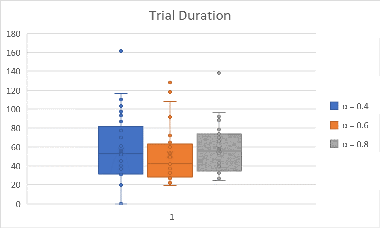
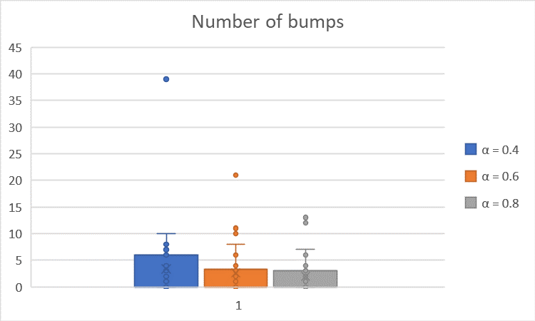
The average is summarized in the table below (the times are in seconds):

Parameter Combination	Ave. Trial Duration	Ave. Number of Bumps
$α = 0.4 \quad (β = 8, γ = 0.9)$	$56.03$	$3.40$
$α = 0.6 \quad (β = 8, γ = 0.9)$	$52.36$	$2.60$
$α = 0.8 \quad (β = 8, γ = 0.9)$	$58.01$	$1.97$

We observe that as $α$ increases, the trial duration over the 30 trials is more stable (as shown in the plot, the data stretch across a smaller range), and the number of bumps decreases. This is because $α$ is the learning rate, and the bigger $α$ is, the quicker the robot learns. In this case, with bigger $α$, the moren the robot’s learning depends on previous trials, and thus make the trial duration over 30 trials more stable/concentrated.

$β$ Test

Then, we test the impact of the parameter $β$ by comparing three different combinations:

(1) $α = 0.4, β = 0.1, γ = 0.9$; (2) $α = 0.4, β = 1, γ = 0.9$; (3) $α = 0.4, β = 8, γ = 0.9$.

The boxplots of the trial duration and number of bump-into-wall are shown below:

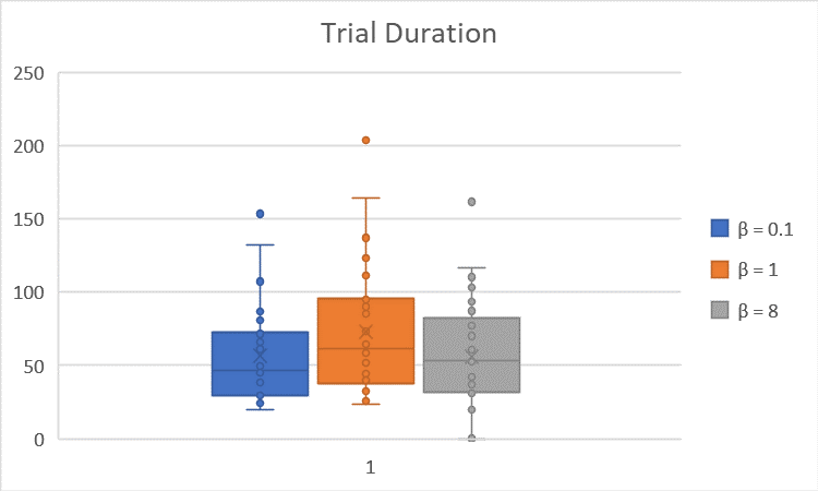
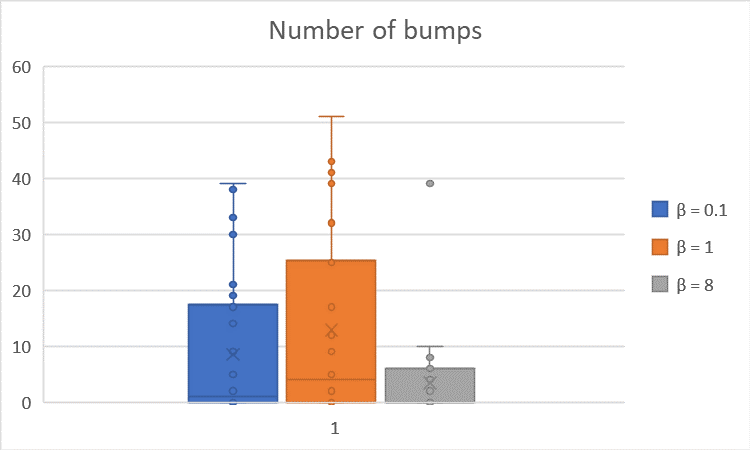
The averages are summarized in the table below:

Parameter Combination	Ave. Trial Duration	Ave. Number of Bumps
$β = 0.1 \quad (α = 0.4, γ = 0.9)$	$56.57$	$8.53$
$β = 1 \quad (α = 0.4, γ = 0.9)$	$73.23$	$12.90$
$β = 8 \quad (α = 0.4, γ = 0.9)$	$56.03$	$3.40$

Theoretically, $β$ is an exploration-exploitation trade-off parameter: for $β$ ≥ 0, the bigger $β$ is, the more the robot tends to exploit the strategy that the robot deems to be the best one according to its estimations; with small $β$, the robot do not choose necessarily the strategy that is deemed to be the best so far. However, we did not see the effect of the $β$ parameter in the simulations because of the fact that whenever $β$ is little and the robot tries to explore strategies irrespective of their Q-values (the robot’s internal estimate of values of the strategies), it is negatively reinforced if it bumps into a wall for instance: so around the walls, the Q-value of the wallFollower gets better and better compared to the one of the guidance strategy, and however little $β$ is, it is not enough to compensate the gap between the two Q-values: the robot ends up choosing greedily again.

$γ$ Test

Finally, we test the impact of the parameter $γ$ by comparing three different combinations:

(1) $α = 0.4, β = 8, γ = 0.1$; (2) $α = 0.4, β = 8, γ = 0.5$; (3) $α = 0.4, β = 8, γ = 0.9$.

The boxplots of the trial duration and number of bump-into-wall are shown below:

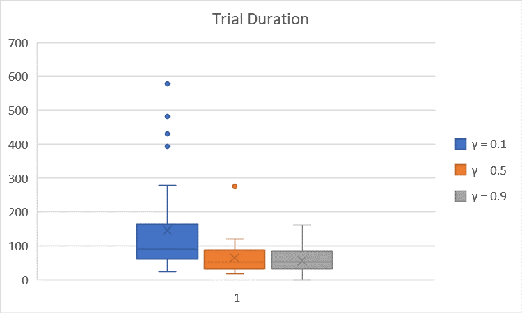
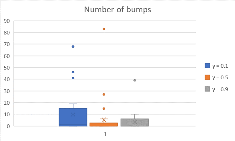
The average is summarized in the table below (times in seconds):

Parameter Combination	Ave. Trial Duration	Ave. Number of Bumps
$γ = 0.1 \quad (α = 0.4, β = 8)$	$145.91$	$9.8$
$γ = 0.5 \quad (α = 0.4, β = 8)$	$65.15$	$5.4$
$γ = 0.9 \quad (α = 0.4, β = 8)$	$56.07$	$3.4$

We observe that $γ$ = $0.1$ leads to significantly longer trial duration and higher number of bumps; $γ = 0.9$ results in a slightly longer trial duration and slightly higher number of bumps than $γ = 0.5$. This is because, $γ$ determines a tradeoff between state exploration (i.e. exploring farther states) and state exploitation/greediness (i.e. don’t really considering farther much in the estimation of the current Q-value) when evaluating the Q-values of a pair of state and action. Thus, the smaller the parameter $γ$, the less the robot takes into account farther state in the Q-value of a state-action pair, which leads to the robot tending to exploit the closest state associated with a (strictly) positive reward (even if there might be a state farther on which a given action leads to a bigger reward). Thus, $γ = 0.1$ could lead to very inefficient choices of the robot, $γ = 0.9$ might lead to some resource waste due to the exploration choice, and $γ = 0.5$ can provide a good balance between the state exploration and the state exploitation.

Here are some gifs from various qlearning simulations with the parameters $α = 0.4, β = 8, γ = 0.1$:

At trial 1

---

At trial 96

---

At trial 101

---

At trial 106

---

At trial 107

---