Problem Set 1: Gaussian Neuronal Noise & Discriminability

Problem 1: Gaussian Neuronal Noise

Suppose we’re trying to read out the stimulus $x$ from the activity of the population of two neurons. Unlike the case of poisson neurons, considered in class, we assume that the neuronal noise is Gaussian.

Namely, the single trial neuronal responses $s_n$ (for $n = 1, 2$) are drawn from a Gaussian distribution centered at the stimulus-dependent values:

\[s_i \leadsto 𝒩(f_i(x), σ_i^2)\]

The functions $f_i(x)$ are called tuning curves.

Show that if the tuning curves are linear wrt $x$ and if there is no prior knowledge about the stimulus, then the posterior distribution over the stimuli $x$ is Gaussian.

Let’s assume that

• $f_i(x) = α_i x$, for $i = 1, 2$
• there is no prior knowledge about the stimulus

Then

\[p(x \mid s_1, s_2) = \frac{p(s_1, s_2 \mid x) \, p(x)}{p(s_1, s_2)} = \text{const} × (\underbrace{p(s_1 \mid x) × p(s_2 \mid x)}_{\text{independent Gaussian variables}}) \\ = \text{const} × \left(\frac{1}{\sqrt{2 π σ_1^2}} \, \exp\left(- \frac{(s_1 - α_1 x)^2}{2 σ_1^2}\right) × \frac{1}{\sqrt{2 π σ_2^2}} \, \exp\left(- \frac{(s_2-α_2 x)^2}{2 σ_2^2}\right)\right) \\ = \text{const'} × \left(\frac{1}{\sqrt{2 π (σ_1 σ_2)^2}} \, \exp\left(- \frac 1 2 \left( \frac{(s_1 - α_1 x)^2}{σ_1^2} + \frac{(s_2-α_2 x)^2}{σ_2^2}\right)\right)\right) \\ = \text{const'} × \left(\frac{1}{\sqrt{2 π (σ_1 σ_2)^2}} \, \exp\left(- \frac 1 2 \frac{σ_2^2 (s_1 - α_1 x)^2 + σ_1^2 (s_2 - α_2 x)^2}{(σ_1 σ_2)^2}\right)\right) \\\]

is Gaussian, since we can check that:

\[𝒩(μ_1, σ_1^2) 𝒩(μ_2, σ_2^2) \propto 𝒩\left(μ, σ\right) \text{ where } \begin{cases} μ = \frac{μ_1 σ_2^2 + μ_2 σ_1^2}{σ_1^2 + σ_2^2} \\ \frac 1 {σ^2} = \frac 1 {σ_1^2} + \frac 1 {σ_2^2} \end{cases}\]

What is the mean and the variance of the posterior? (No prior knowledge about the stimulus implies that the prior is a uniform distribution over a very wide range)

\[p(s_i \mid x) = \frac{1}{\sqrt{2 π σ_i^2}} \, \exp\left(- \frac{(s_i - f_i(x))^2}{2 σ_i^2}\right)\]

According to the previous question:

•  The new mean is: \(\cfrac{\frac{s_1}{α_1} \frac{σ_2^2}{α_2^2} + \frac{s_2}{α_2} \frac{σ_1^2}{α_1^2}}{\frac{σ_2^2}{α_2^2} + \frac{σ_1^2}{α_2^2}}\)

•  The new variance is: \(\left(\frac{α_2^2}{σ_2^2} + \frac{α_1^2}{σ_1^2}\right)^{-1}\)

Does the answer make sense to you? Which of the two neurons provides the more information about the stimulus (whose response has a stronger weight in inferring the stimulus)?

Thanks to the ratios $\frac{σ_i}{α_i}$, multiplying $σ_i$ and $α_i$ by the same constant won’t change anything.

So if we plot $p(s_i \mid x)$ as a function of $s_i$: multiplying the mean by $k$ leads to the variance being multiplied by $k$.

These ratios make sense indeed, since if you double the number of neurons, you double the variance.

If $σ_1/α_1 » σ_2/α_2$, then the new mean is converges $\frac{s_2}{α_2}$: so the first neuron doesn’t contribute anymore (the other one is more informative).

The smaller ratio $σ_1/α_1$, the more informative the neuron is.

The mean $p(x \mid s_1, s_2)$ of two joined Gaussians $p(x \mid s_1)$ and $p(x \mid s_2)$ is a weighted sum of the means of the two Gaussians: the smaller the variance of one Gaussian, the bigger its weight in the weighted sum.

Problem 2

Suppose you have measured a spike-count $s$ of a single neuron in response to a stimulus $x$. You know, that the stimulus could have been either $x = x_0$ or $x = x_0 + δx$, where $δx$ is small.

You are trying to guess which of the two stimuli was presented.

Consider the expression:

\[D(x_0, s) ≝ \frac{p(s \mid x_0)}{p(s \mid x_0 + δx)} + \frac{p(s \mid x_0 + δx)}{p(s \mid x_0)} - 2\]

We will refer to $D(x,s)$ as discriminability.

a).

Can $D(x_0, s)$ be negative?

The function

\[f : \begin{cases} ℝ^\ast_+ &⟶ ℝ^\ast_+ \\ y &⟼ y + \frac{1}{y} \end{cases}\]

is convex (indeed: $f^{\prime \prime}(x) = \frac{2}{y^3} > 0$), so its minimum is reached at $y_\ast ∈ ℝ^\ast_+$ such that:

\[f'(y_\ast) = 0 ⟺ 1 - \frac{1}{y_\ast^2} = 0\\ ⟺ y_\ast = 1\]

And its global minimum is equal to $f(1) = 2$.

So $D(x_0, s) ≝ f\left(\frac{p(s \mid x_0)}{p(s \mid x_0 + δx)}\right) - 2 ≥ 0$ cannot be (stricly) negative.

What does $D(x_0, s) = 0$ indicate?

\[\begin{align*} &\quad D(x_0, s) = 0 \\ ⟺ &\quad f\left(\frac{p(s \mid x_0)}{p(s \mid x_0 + δx)}\right) = 2 \\ ⟺ &\quad \frac{p(s \mid x_0)}{p(s \mid x_0 + δx)} = 1\\ ⟺ &\quad p(s \mid x_0) = p(s \mid x_0 + δx) \end{align*}\]

Can you convince yourself that the larger $D(x_0, s)$ is, the more information the measurement $s$ provides about the stimulus $x$?

The graph of $f$ is as follows:

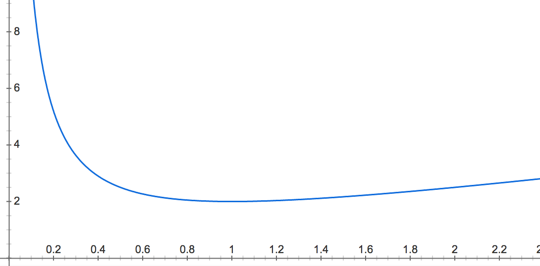
Clearly:

• \[f(y) ≝ y + \frac{1}{y} \sim_{0^+} \frac{1}{y} \xrightarrow[y \to 0^+]{} +∞\]
• \[f(y) ≝ y + \frac{1}{y} \sim_{+∞} y \xrightarrow[y \to +∞]{} +∞\]

So that $D(x_0, s)$ tends to $+∞$ whenever:

• \[y ≝ \frac{p(s \mid x_0)}{p(s \mid x_0 + δx)} ⟶ 0^+, \text{ i.e. } p(s \mid x_0 + δx) >> p(s \mid x_0)\]

or

• \[y ≝ \frac{p(s \mid x_0)}{p(s \mid x_0 + δx)} ⟶ +∞, \text{ i.e. } p(s \mid x_0) >> p(s \mid x_0 + δx)\]

The larger $D(x_0,s)$, the more information the measurement $s$ provides about the relative size of $p(s \mid x_0)$ and $p(s \mid x_0 + δx)$, and thus about $x$.

Using Taylor expansion in $δx$, derive the leading order contribution to $D(x_0, s)$.

Assuming $p$ is sufficiently regular:

\[p(s \mid x_0 + δx) ≃ p(s \mid x_0) + δx \left[\frac{\partial p(s \mid x)}{\partial x}\right]_{x=x_0} + \frac{δx^2}{2} \left[ \frac{\partial^2 p(s \mid x)}{\partial x^2}\right]_{x=x_0}\]

So that

\[\begin{align*} D(x_0, s) & = \frac{p(s \mid x_0)}{p(s \mid x_0 + δx)} + \frac{p(s \mid x_0 + δx)}{p(s \mid x_0)} - 2 \\ & ≃ \frac{1}{1+ \frac{1}{p(s \mid x_0)} \left(δx \left[\frac{\partial p(s \mid x)}{\partial x}\right]_{x=x_0} + \frac{δx^2}{2} \left[ \frac{\partial^2 p(s \mid x)}{\partial x^2}\right]_{x=x_0}\right)} + 1 + δx \cfrac{\left[\frac{\partial p(s \mid x)}{\partial x}\right]_{x=x_0}}{p(s \mid x_0)} + \cfrac{\frac{δx^2}{2} \left[ \frac{\partial^2 p(s \mid x)}{\partial x^2}\right]_{x=x_0}}{p(s \mid x_0)} -2 \\ & ≃ 1 - \frac{1}{p(s \mid x_0)} \left(δx \left[\frac{\partial p(s \mid x)}{\partial x}\right]_{x=x_0} + \frac{δx^2}{2} \left[ \frac{\partial^2 p(s \mid x)}{\partial x^2}\right]_{x=x_0}\right) + \left(\frac{1}{p(s \mid x_0)} \left(δx \left[\frac{\partial p(s \mid x)}{\partial x}\right]_{x=x_0} + \frac{δx^2}{2} \left[ \frac{\partial^2 p(s \mid x)}{\partial x^2}\right]_{x=x_0}\right)\right)^2 + 1 + δx \cfrac{\left[\frac{\partial p(s \mid x)}{\partial x}\right]_{x=x_0}}{p(s \mid x_0)} + \cfrac{\frac{δx^2}{2} \left[ \frac{\partial^2 p(s \mid x)}{\partial x^2}\right]_{x=x_0}}{p(s \mid x_0)} -2\\ &= \frac{1}{p(s \mid x_0)^2} \left(δx \left[\frac{\partial p(s \mid x)}{\partial x}\right]_{x=x_0} + \frac{δx^2}{2} \left[ \frac{\partial^2 p(s \mid x)}{\partial x^2}\right]_{x=x_0}\right)^2 \end{align*}\]

So the second order is the dominating one.

In the case when $p(s \mid x)$ is Gaussian ($p(s \mid x) \sim 𝒩(x, σ^2)$), what outcomes $s$ are more informative about $x$?

(Not done yet)