Exercise Sheet 5: Perceptrons and Hopfield networks
Exercise Sheet 5: Perceptrons and Hopfield networks
Younesse Kaddar
\[\newcommand{\T}{ {\raise{0.7ex}{\intercal}}} \newcommand{\sign}{\textrm{sign}}\]1. Peceptrons
Consider the following two sets of two-dimensional patterns:
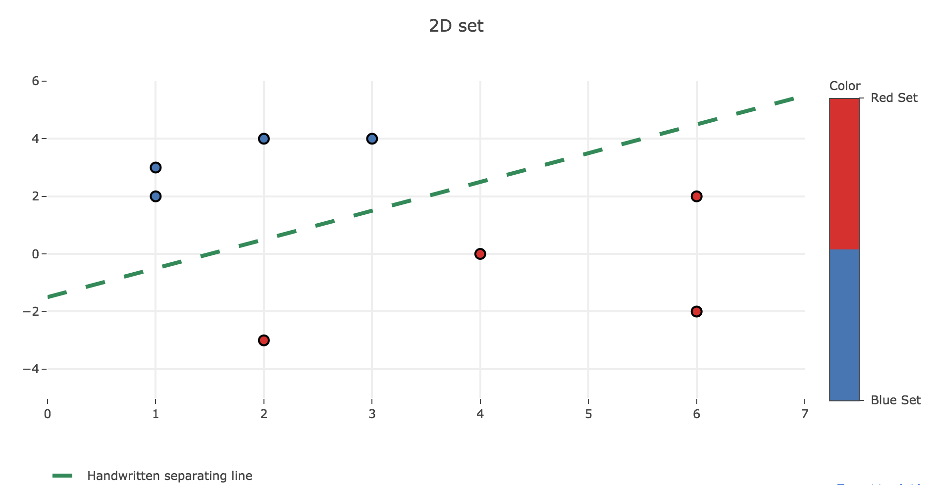
\[𝒟_{\text{blue}} = \lbrace (1, 2), (1, 3), (3, 4), (2, 4) \rbrace\\ 𝒟_{\text{red}} = \lbrace (4, 0), (6, 2), (2, -3), (6, -2) \rbrace\]a. Are the two sets linearly separable? If they are, use a preceptron rule to find a readout weight vector that allows a binary neuron to classify the two sets in two different categories
The two sets are easily seen to be separable, by the line whose equation is $y = x - 1.5$ for example, as shown in the figure below:
The algorithm using the perceptron rule is the following one (in pseudo-code):
n_trials = 8

# Color of the points: 0 ≡ blue / 1 ≡ red
Y → [0, 0, 0, 0, 1, 1, 1, 1]

# Data points
X → [[1,2],[1,3],[3,4],[2,4],[4,0],[6,2],[2,-3],[6,-2]]

# Initialize the weight vector
w → (1, 1)

while True:
    # is the weight still changing? To end the loop
    still_changing → False

    for 1 ≤ k ≤ nb_trials:
        # output = 1 if the scalar product is > 0, else 0
        output → H(⟨w, X[k]⟩)

        w_new → w + (Y[k]-output)*X[k]

        if w_new != w:
            still_changing = True

        w → w_new

    if not still_changing:
        break

return w
Let us run it on our 2D-data set:
| Step | $w$ | $k$ | $x^{(k)}$ | $y^{(k)}$ | $⟨w, x^{(k)}⟩$ | output |
$y_k$ - output |
$w_{\text{new}}$ |
|---|---|---|---|---|---|---|---|---|
| $(1, 1)$ | ||||||||
| $1$ | $(1, 1)$ | $1$ | $(1, 2)$ | $0$ | $1 \cdot 1+ 1 \cdot 2\ = 3$ | $1$ | $-1$ | $(1, 1)-(1, 2)\ = (0, -1)$ |
| $1$ | $(0, -1)$ | $2$ | $(1, 3)$ | $0$ | $0 \cdot 1 - 1 \cdot 3\ = -3$ | $0$ | $0$ | $(0, -1)$ |
| $1$ | $(0, -1)$ | $3$ | $(3, 4)$ | $0$ | $0 \cdot 3 - 1 \cdot 4\ = -4$ | $0$ | $0$ | $(0, -1)$ |
| $1$ | $(0, -1)$ | $4$ | $(2, 4)$ | $0$ | $0 \cdot 2 - 1 \cdot 4\ = -4$ | $0$ | $0$ | $(0, -1)$ |
| $1$ | $(0, -1)$ | $5$ | $(4, 0)$ | $1$ | $0 \cdot 4 - 1 \cdot 0\ = 0$ | $1$ | $0$ | $(0, -1)$ |
| $1$ | $(0, -1)$ | $6$ | $(6, 2)$ | $1$ | $0 \cdot 6 - 1 \cdot 2\ = -2$ | $0$ | $1$ | $(0, -1)+(6, 2)\=(6, 1)$ |
| $1$ | $(6, 1)$ | $7$ | $(2, -3)$ | $1$ | $6 \cdot 2 - 1 \cdot 3\= 9$ | $1$ | $0$ | $(6, 1)$ |
| $1$ | $(6, 1)$ | $8$ | $(6, -2)$ | $1$ | $6 \cdot 6 - 1 \cdot 2\= 34$ | $1$ | $0$ | $(6, 1)$ |
| $2$ | $(6, 1)$ | $9$ | $(1, 2)$ | $0$ | $6 \cdot 1 + 1 \cdot 2\= 8$ | $1$ | $-1$ | $(5, -1)$ |
| $2$ | $(5, -1)$ | $10$ | $(1, 3)$ | $0$ | $5 \cdot 1 - 1 \cdot 3\= 2$ | $1$ | $-1$ | $(5, -1)-(1, 3)\=(4, -4)$ |
| $2$ | $(4, -4)$ | $11$ | $(3, 4)$ | $0$ | $4 \cdot 3 - 4 \cdot 4\= -4$ | $0$ | $0$ | $(4, -4)$ |
| $2$ | $(4, -4)$ | $12$ | $(2, 4)$ | $0$ | $4 \cdot 2 - 4 \cdot 4\= -8$ | $0$ | $0$ | $(4, -4)$ |
| $2$ | $(4, -4)$ | $13$ | $(4, 0)$ | $1$ | $4 \cdot 4 - 4 \cdot 0\= 16$ | $1$ | $0$ | $(4, -4)$ |
| $2$ | $(4, -4)$ | $14$ | $(6, 2)$ | $1$ | $4 \cdot 6 - 4 \cdot 2\= 16$ | $1$ | $0$ | $(4, -4)$ |
| $2$ | $(4, -4)$ | $15$ | $(2, -3)$ | $1$ | $4 \cdot 2 + 4 \cdot 3\= 20$ | $1$ | $0$ | $(4, -4)$ |
| $2$ | $(4, -4)$ | $16$ | $(6, -2)$ | $1$ | $4 \cdot 6 + 4 \cdot 2\= 32$ | $1$ | $0$ | $(4, -4)$ |
| $3$ | $(4, -4)$ | $17$ | $(1, 2)$ | $0$ | $4 \cdot 1 - 4 \cdot 2\= -4$ | $0$ | $0$ | $(4, -4)$ |
| $3$ | $(4, -4)$ | $18$ | $(1, 3)$ | $0$ | $4 \cdot 1 - 4 \cdot 3\= -8$ | $0$ | $0$ | $(4, -4)$ |
| $3$ | $(4, -4)$ | $19$ | $(3, 4)$ | $0$ | $4 \cdot 3 - 4 \cdot 4\= -4$ | $0$ | $0$ | $(4, -4)$ |
| $3$ | $(4, -4)$ | $20$ | $(2, 4)$ | $0$ | $4 \cdot 2 - 4 \cdot 4\= -8$ | $0$ | $0$ | $(4, -4)$ |
| $3$ | $(4, -4)$ | $21$ | $(4, 0)$ | $1$ | $4 \cdot 4 - 4 \cdot 0\= 16$ | $1$ | $0$ | $(4, -4)$ |
| $3$ | $(4, -4)$ | $22$ | $(6, 2)$ | $1$ | $4 \cdot 6 - 4 \cdot 2\= 16$ | $1$ | $0$ | $(4, -4)$ |
| $3$ | $(4, -4)$ | $23$ | $(2, -3)$ | $1$ | $4 \cdot 2 + 4 \cdot 3\= 20$ | $1$ | $0$ | $(4, -4)$ |
| $3$ | $(4, -4)$ | $24$ | $(6, -2)$ | $1$ | $4 \cdot 6 + 4 \cdot 2\= 32$ | $1$ | $0$ | $(4, -4)$ |
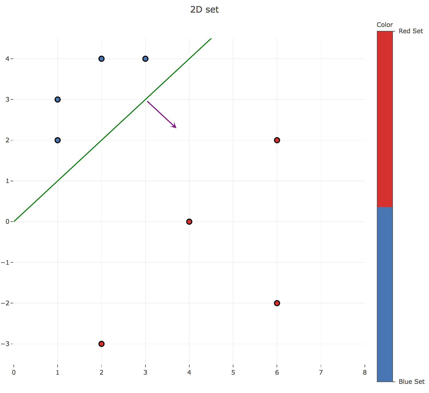
The algorithm stops at the end of the third step because the readout weight vector $w ≝ (4, -4)$ hasn’t changed throughout this step: all the points have finally been correctly classified.
Therefore: the decision boundary turns out to the line given by the equation:
\[\underbrace{w_0}_{≝ 4} x + \underbrace{w_1}_{≝ -4} y = 0 ⟺ y = x\]which can easily be checked on the data points: a point $(x, y)$ is classified as red (resp. blue) if and only if $x > y$ (resp. $x ≤ y$).
Here is the resulting separating line (in green), along with the normalized readout weight vector $w$ (in purple):
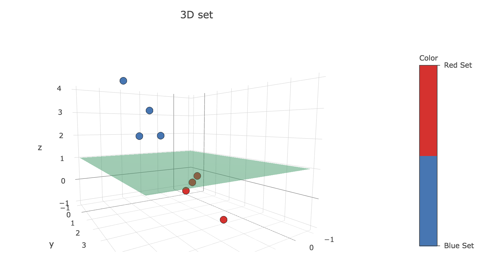
b. Repeat the exercise with the following two sets of three-dimensional patterns:
\[𝒟_{\text{blue}} = \lbrace (2, 1, 2), (3, 2, 3), (4, 2, 4), (3, 1, 2) \rbrace\\ 𝒟_{\text{red}} = \lbrace (1, 4, -1), (2, 3, 0), (1, 2, 0), (0, 1, 0) \rbrace\]Again, the data sets are seen to be linearly separable (with the $z = 1$ plane for instance):
This time, the values are initialized as follows:
n_trials = 8

# Color of the points: 0 ≡ blue / 1 ≡ red
Y → [0, 0, 0, 0, 1, 1, 1, 1]

# Data points
X → [[2,1,2],[3,2,3],[4,2,4],[3,1,2],[1,4,-1],[2,3,0],[1,2,0],[0,1,0]]

# Initialize the weight vector
w → (1, 1, 1)
Let us run the algorithm on this 3D-data set:
| Step | $w$ | $k$ | $x^{(k)}$ | $y^{(k)}$ | $⟨w, x^{(k)}⟩$ | output |
$y_k$ - output |
$w_{\text{new}}$ |
|---|---|---|---|---|---|---|---|---|
| $(1, 1, 1)$ | ||||||||
| $1$ | $(1, 1, 1)$ | $1$ | $(2, 1, 2)$ | $0$ | $1 \cdot 2 + 1 \cdot 1 + 1 \cdot 2 \ = 5$ | $1$ | $-1$ | $(1, 1, 1)-(2, 1, 2)\ = (-1, 0, -1)$ |
| $1$ | $(-1, 0, -1)$ | $2$ | $(3, 2, 3)$ | $0$ | $-1 \cdot 3 + 0 \cdot 2 - 1 \cdot 3\ = -6$ | $0$ | $0$ | $(-1, 0, -1)$ |
| $1$ | $(-1, 0, -1)$ | $3$ | $(4, 2, 4)$ | $0$ | $-1 \cdot 4 + 0 \cdot 2 - 1 \cdot 4\ = -8$ | $0$ | $0$ | $(-1, 0, -1)$ |
| $1$ | $(-1, 0, -1)$ | $4$ | $(3, 1, 2)$ | $0$ | $-1\cdot 3 + 0 \cdot 1 - 1 \cdot 2\ = -5$ | $0$ | $0$ | $(-1, 0, -1)$ |
| $1$ | $(-1, 0, -1)$ | $5$ | $(1, 4, -1)$ | $1$ | $-1 \cdot 1 + 0 \cdot 4 + 1 \cdot 1\ = 0$ | $1$ | $0$ | $(-1, 0, -1)$ |
| $1$ | $(-1, 0, -1)$ | $6$ | $(2, 3, 0)$ | $1$ | $-1 \cdot 2 + 0 \cdot 3 - 1 \cdot 0\ = -2$ | $0$ | $1$ | $(-1, 0, -1)+(2, 3, 0)\=(1, 3, -1)$ |
| $1$ | $(1, 3, -1)$ | $7$ | $(1, 2, 0)$ | $1$ | $1 \cdot 1 + 3 \cdot 2 - 1 \cdot 0\= 7$ | $1$ | $0$ | $(1, 3, -1)$ |
| $1$ | $(1, 3, -1)$ | $8$ | $(0, 1, 0)$ | $1$ | $1 \cdot 0 + 3 \cdot 1 - 1 \cdot 0\= 3$ | $1$ | $0$ | $(1, 3, -1)$ |
| $2$ | $(1, 3, -1)$ | $9$ | $(2, 1, 2)$ | $0$ | $1 \cdot 2 + 3 \cdot 1 - 1 \cdot 2\= 3$ | $1$ | $-1$ | $(1, 3, -1) - (2, 1, 2)\= (-1, 2, -3)$ |
| $2$ | $(-1, 2, -3)$ | $10$ | $(3, 2, 3)$ | $0$ | $-1 \cdot 3 + 2 \cdot 2 - 3 \cdot 3\= -8$ | $0$ | $0$ | $(-1, 2, -3)$ |
| $2$ | $(-1, 2, -3)$ | $11$ | $(4, 2, 4)$ | $0$ | $-1 \cdot 4 + 2 \cdot 2 - 3 \cdot 4\= -12$ | $0$ | $0$ | $(-1, 2, -3)$ |
| $2$ | $(-1, 2, -3)$ | $12$ | $(3, 1, 2)$ | $0$ | $-1 \cdot 3 + 2 \cdot 1 - 3 \cdot 2\= -7$ | $0$ | $0$ | $(-1, 2, -3)$ |
| $2$ | $(-1, 2, -3)$ | $13$ | $(1, 4, -1)$ | $1$ | $-1 \cdot 1 + 2 \cdot 4 + 3 \cdot 1\= 10$ | $1$ | $0$ | $(-1, 2, -3)$ |
| $2$ | $(-1, 2, -3)$ | $14$ | $(2, 3, 0)$ | $1$ | $-1 \cdot 2 + 2 \cdot 3 - 3 \cdot 0\= 4$ | $1$ | $0$ | $(-1, 2, -3)$ |
| $2$ | $(-1, 2, -3)$ | $15$ | $(1, 2, 0)$ | $1$ | $-1 \cdot 1 + 2 \cdot 2 - 3 \cdot 0\= 3$ | $1$ | $0$ | $(-1, 2, -3)$ |
| $2$ | $(-1, 2, -3)$ | $16$ | $(0, 1, 0)$ | $1$ | $-1 \cdot 0 + 2 \cdot 1 - 3 \cdot 0\= 2$ | $1$ | $0$ | $(-1, 2, -3)$ |
| $3$ | $(-1, 2, -3)$ | $17$ | $(2, 1, 2)$ | $0$ | $-1 \cdot 2 + 2 \cdot 1 - 3 \cdot 2\= -6$ | $0$ | $0$ | $(-1, 2, -3)$ |
| $3$ | $(-1, 2, -3)$ | $18$ | $(3, 2, 3)$ | $0$ | $-1 \cdot 3 + 2 \cdot 2 - 3 \cdot 3\= -8$ | $0$ | $0$ | $(-1, 2, -3)$ |
| $3$ | $(-1, 2, -3)$ | $19$ | $(4, 2, 4)$ | $0$ | $-1 \cdot 4 + 2 \cdot 2 - 3 \cdot 4\= -12$ | $0$ | $0$ | $(-1, 2, -3)$ |
| $3$ | $(-1, 2, -3)$ | $20$ | $(3, 1, 2)$ | $0$ | $-1 \cdot 3 + 2 \cdot 1 - 3 \cdot 2\= -7$ | $0$ | $0$ | $(-1, 2, -3)$ |
| $3$ | $(-1, 2, -3)$ | $21$ | $(1, 4, -1)$ | $1$ | $-1 \cdot 1 + 2 \cdot 4 + 3 \cdot 1\= 10$ | $1$ | $0$ | $(-1, 2, -3)$ |
| $3$ | $(-1, 2, -3)$ | $22$ | $(2, 3, 0)$ | $1$ | $-1 \cdot 2 + 2 \cdot 3 - 3 \cdot 0\= 4$ | $1$ | $0$ | $(-1, 2, -3)$ |
| $3$ | $(-1, 2, -3)$ | $23$ | $(1, 2, 0)$ | $1$ | $-1 \cdot 1 + 2 \cdot 2 - 3 \cdot 0\= 3$ | $1$ | $0$ | $(-1, 2, -3)$ |
| $3$ | $(-1, 2, -3)$ | $24$ | $(0, 1, 0)$ | $1$ | $-1 \cdot 0 + 2 \cdot 1 - 3 \cdot 0\= 2$ | $1$ | $0$ | $(-1, 2, -3)$ |
Again, the algorithm stops at the end of the third step because the readout weight vector $w ≝ (-1, 2, -3)$ hasn’t changed throughout this step: all the points have been correctly classified.
The decision boundary is the plane given by the equation:
\[\underbrace{w_0}_{≝ -1} x + \underbrace{w_1}_{≝ 2} y + \underbrace{w_2}_{≝ -3} z = 0 ⟺ z = \frac 2 3 y - \frac 1 3 x\]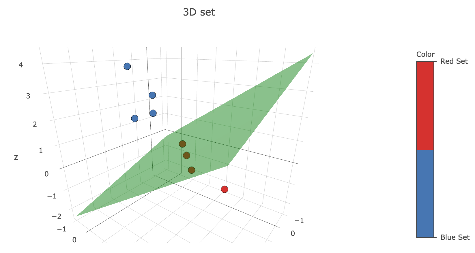
c. Optional: Code the perceptron rule in a computer, and use the datasets of exercises a) and b) to check the validity of your answers. Please attach your code and the results obtained.
Here is a python implementation:
def perceptron_rule(X, Y):
    nb_trials, dimension = X.shape
    w = np.ones(X.shape[1])
    w_values = [np.copy(w)]

    while True:
        # is the readout vector still changing?
        # (to halt the loop, in case it isn't)
        still_changing = False

        for i in range(nb_trials):
            w += (Y[i]-int(w.dot(X[i])>=0))*X[i]

            if np.any(w_values[-1] != w):
                still_changing = True
            w_values.append(np.copy(w))

        if not still_changing:
            break

    # Returning all the readout weight vectors,
    # except those of the last step
    # (throughout which the readout vector didn't change)
    return np.array(w_values[:-nb_trials])
Here are the outputs:
-
for 2D-data sets:
  array([[ 1.,  1.],
     [ 0., -1.],
     [ 0., -1.],
     [ 0., -1.],
     [ 0., -1.],
     [ 0., -1.],
     [ 6.,  1.],
     [ 6.,  1.],
     [ 6.,  1.],
     [ 5., -1.],
     [ 4., -4.],
     [ 4., -4.],
     [ 4., -4.],
     [ 4., -4.],
     [ 4., -4.],
     [ 4., -4.],
     [ 4., -4.]])
which gives the following successive decision boundaries (the successive normalized readout vectors are plotted in purple) throughout the iterations of the main loop:
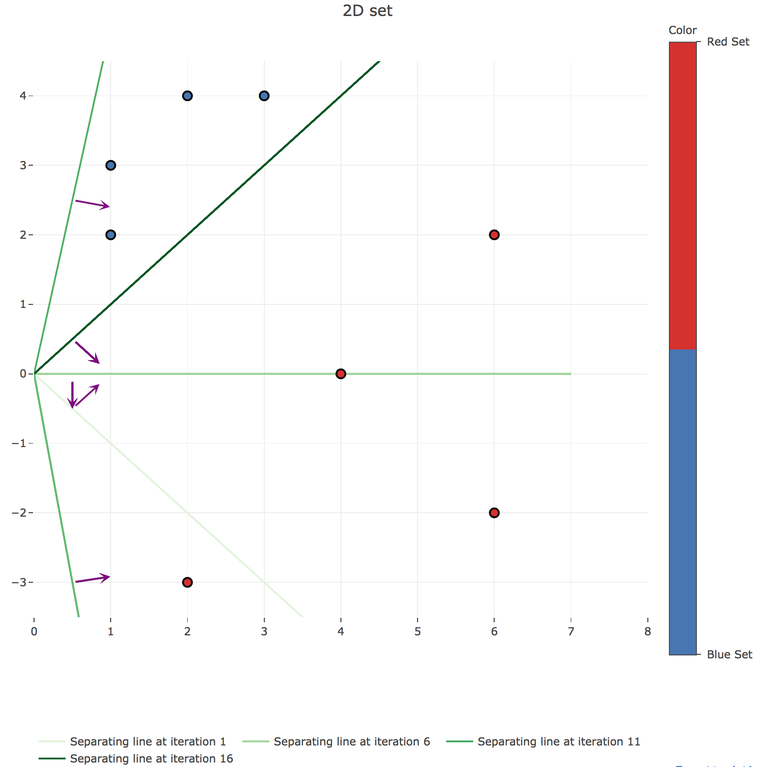
Figure 1.c.1. - Plot of the successive decision boundaries thoughout the algorithm (with their corresponding normalized readout vectors in purple) -
for the 3D-one:
  array([[ 1.,  1.,  1.],
     [-1.,  0., -1.],
     [-1.,  0., -1.],
     [-1.,  0., -1.],
     [-1.,  0., -1.],
     [-1.,  0., -1.],
     [ 1.,  3., -1.],
     [ 1.,  3., -1.],
     [ 1.,  3., -1.],
     [-1.,  2., -3.],
     [-1.,  2., -3.],
     [-1.,  2., -3.],
     [-1.,  2., -3.],
     [-1.,  2., -3.],
     [-1.,  2., -3.],
     [-1.,  2., -3.],
     [-1.,  2., -3.]])
which gives the following successive decision planes throughout the iterations of the main loop:
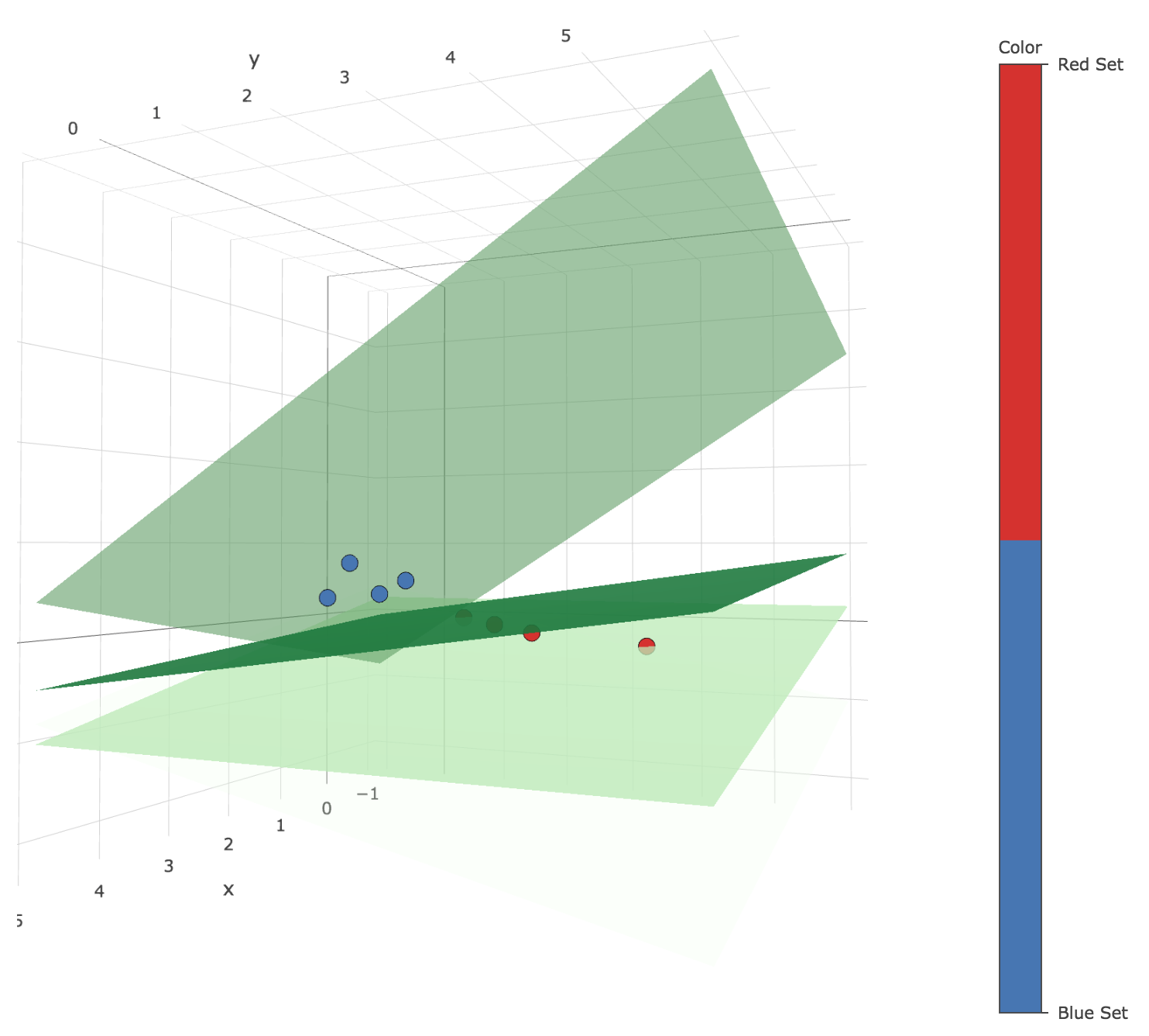
Figure 1.c.1. - Plot of the successive decision planes thoughout the algorithm (the darker, the higher the corresponding iteration number)
which is exactly what we’ve computed by hand.
2. Hopfield networks
a. Consider a recurrent network of five binary neurons. Use the Hopfield rule to determine the synaptic weights of the network so that the pattern $ξ^\ast = (1, -1, -1, 1, -1) ∈ 𝔐_{1, 5}(ℝ)$ is memorized. Show explicitly that $ξ^\ast$ is a fixed point of the dynamics.
According to the Hopfield rule, the weights of the synaptic matrix $W ≝ (w_{ij})_{1 ≤ i, j ≤ 5}$ are to be set to:
\[w_{ij} ≝ \frac 1 5 ξ^\ast_i ξ^\ast_j\]The resulting synaptic matrix is:
\[W ≝ \frac 1 5 {ξ^\ast}^\T ξ^\ast = \frac 1 5 \begin{pmatrix} 1 & -1 & -1 & 1 & -1 \\ -1 & 1 & 1 & -1 & 1 \\ -1 & 1 & 1 & -1 & 1 \\ 1 & -1 & -1 & 1 & -1 \\ -1 & 1 & 1 & -1 & 1 \\ \end{pmatrix}\]As a matter of fact:
\[\begin{align*} \sign\left(W {ξ^\ast}^\T\right) & = \sign\left(\frac 1 5 \left({ξ^\ast}^\T ξ^\ast\right) {ξ^\ast}^\T\right) \\ & = \sign\left(\frac 1 5 {ξ^\ast}^\T \left(ξ^\ast {ξ^\ast}^\T\right)\right) &&\text{(because the matrix product is associative)}\\ &= \sign\Bigg(\frac 1 5 {ξ^\ast}^\T \overbrace{\Bigg(\sum\limits_{ i=1 }^5 \underbrace{(ξ^\ast_i)^2}_{= \; 1}\Bigg)}^{= \; 5}\Bigg) \\ &= \sign\left({ξ^\ast}^\T\right) \\ &= {ξ^\ast}^\T &&\text{(because } ξ^\ast ∈ \lbrace -1, 1 \rbrace^5 \text{ )} \end{align*}\]So ${ξ^\ast}^\T$ ($ξ^\ast$ by abuse of notation) is indeed a fixed point of the dynamics.
b. What is the output of the network if the dynamics start from the initial state $ξ = (1, -1, -1, 1, -1)$?
As shown before, if the dynamics start from the initial state $ξ = (1, -1, -1, 1, -1)$, the ouput is the same state $(1, -1, -1, 1, -1)$ as it is a fixed point.
Based on the teacher’s remark in class, I think the question was rather meant to be about the initial state being $ξ ≝ (-1, 1, 1, -1, 1) = - ξ^\ast$
In this case, retrieving last computation:
\[\begin{align*} \sign\left(W ξ^\T\right) & = \sign\left(\frac 1 5 \left({ξ^\ast}^\T ξ^\ast\right) ξ^\T\right) \\ & = \sign\left(\frac 1 5 \left({ξ^\ast}^\T ξ^\ast\right) (-ξ^\ast)^\T\right) \\ & = \sign\left(- \frac 1 5 \left({ξ^\ast}^\T ξ^\ast\right) {ξ^\ast}^\T\right) \\ & = - \; \sign\Bigg(\frac 1 5 {ξ^\ast}^\T \underbrace{\left(ξ^\ast {ξ^\ast}^\T\right)}_{= \; 5}\Bigg) &&\text{(because } \sign \text{ is an odd function)}\\ &= - \; \underbrace{\sign\left({ξ^\ast}^\T\right)}_{\rlap{= \; {ξ^\ast}^\T \text{ (cf. the previous question)}}} \\ &= - {ξ^\ast}^\T \\ &= ξ^\T &&\text{(by definition of } ξ \text{ )} \end{align*}\]As a result: $ξ^\T ≝ -{ξ^\ast}^\T$ ($ξ$ by abuse of notation) is also a fixed point of the dynamics.
c. Using the Hopfield rule, modify the synaptic weights so that $η^\ast = (1, 1, -1, -1, -1)$ is also memorized. Verify that both $ξ^\ast$ and $η^\ast$ are fixed points of the dynamics.
This, the Hopfield rule yields:
\[∀ i, j ∈ \lbrace 1, \ldots, 5 \rbrace, \quad w_{ij} ≝ \frac 1 5 (ξ^\ast_i ξ^\ast_j + η^\ast_i η^\ast_j)\]The resulting synaptic matrix is:
\[W ≝ \frac 1 5 ({ξ^\ast}^\T ξ^\ast + {η^\ast}^\T η^\ast) = \frac 2 5 \begin{pmatrix} 1 & 0 & -1 & 0 & -1 \\ 0 & 1 & 0 & -1 & 0 \\ -1 & 0 & 1 & 0 & 1 \\ 0 & -1 & 0 & 1 & 0 \\ -1 & 0 & 1 & 0 & 1 \\ \end{pmatrix}\]As a matter of fact, now:
\[\begin{align*} \sign\left(W {ξ^\ast}^\T\right) & = \sign\left(\frac 1 5 \left({ξ^\ast}^\T ξ^\ast + {η^\ast}^\T η^\ast\right) {ξ^\ast}^\T\right) \\ & = \sign\Big(\underbrace{\frac 1 5 \left({ξ^\ast}^\T ξ^\ast\right) {ξ^\ast}^\T}_{\rlap{= \; {ξ^\ast}^\T \; \text{(cf. previous questions)}}} + \frac 1 5 \left({η^\ast}^\T η^\ast\right) {ξ^\ast}^\T\Big)\\ & = \sign\Big({ξ^\ast}^\T + \frac 1 5 \, {η^\ast}^\T \underbrace{\left(η^\ast {ξ^\ast}^\T\right)}_{\rlap{= \; ⟨η^\ast,\, ξ^\ast⟩ \, = \, \sum\limits_{ i = 1}^5 η^\ast_i ξ^\ast_i \, = \, 1}}\Big)\\ &= \sign\Big({ξ^\ast}^\T + \frac 1 5 {η^\ast}^\T\Big) \\ &\overset{⊛}{=} \sign\left({ξ^\ast}^\T\right) &&\text{(because } \frac 1 5 η^\ast ∈ \left\lbrace - \frac 1 5, \frac 1 5 \right\rbrace^5 \text{: it can't change the sign of } ξ^\ast ∈ \lbrace -1, 1 \rbrace^5 \text{ )} \\ &= {ξ^\ast}^\T \end{align*}\]And likewise:
\[\begin{align*} \sign\left(W {η^\ast}^\T\right) & = \sign\left(\frac 1 5 \left({ξ^\ast}^\T ξ^\ast + {η^\ast}^\T η^\ast\right) {η^\ast}^\T\right) \\ & = \sign\Big(\frac 1 5 \left({ξ^\ast}^\T ξ^\ast\right) {η^\ast}^\T + \frac 1 5 \left({η^\ast}^\T η^\ast\right) {η^\ast}^\T\Big)\\ & = \sign\Big(\frac 1 5 {ξ^\ast}^\T \underbrace{\left(ξ^\ast {η^\ast}^\T\right)}_{= \, ⟨ξ^\ast, \, η^\ast⟩ \, = \, 1} + \frac 1 5 {η^\ast}^\T \underbrace{\left(η^\ast {η^\ast}^\T\right)}_{\rlap{= \, ⟨η^\ast, η^\ast⟩ \, = \, \sum\limits_{ i=1 }^5 (η^\ast_i)^2 \, = \, 5}}\Big)\\ & = \sign\Big(\frac 1 5 \, {ξ^\ast}^\T + {η^\ast}^\T \Big)\\ &\overset{⊛}{=} \sign\left({η^\ast}^\T\right) &&\text{(because } \frac 1 5 ξ^\ast ∈ \left\lbrace - \frac 1 5, \frac 1 5 \right\rbrace^5 \text{: it can't change the sign of } η^\ast ∈ \lbrace -1, 1 \rbrace^5 \text{ )} \\ &= {η^\ast}^\T \end{align*}\]So ${ξ^\ast}^\T$ and ${η^\ast}^\T$ ($ξ^\ast$ and $η^\ast$ by abuse of notation) are both fixed points of the dynamics.
NB: in the computations, we see that the equality $⊛$ is crucial to have ${ξ^\ast}^\T$ and ${η^\ast}^\T$ be fixed points. This stems from the fact that
\[{ξ^\ast}^\T + \frac 1 5 \, {η^\ast}^\T ⟨η^\ast, ξ^\ast⟩ \quad \text{(resp. } {η^\ast}^\T + \frac 1 5 \, {ξ^\ast}^\T ⟨η^\ast, ξ^\ast⟩ \text{ )}\]has the same sign as ${ξ^\ast}^\T$ (resp. ${η^\ast}^\T$), which comes itself from the fact that $\vert ⟨η^\ast, ξ^\ast⟩ \vert < 5$ (note that $\vert ⟨η^\ast, ξ^\ast⟩ \vert ≤ 5$ is a consequence of $η^\ast, ξ^\ast ∈ \lbrace -1, 1 \rbrace^5$, but the latter condition is not enough not ensure that $\vert ⟨η^\ast, ξ^\ast⟩ \vert < 5$).
So a sufficient condition for any $ξ, η ∈ \lbrace -1, 1 \rbrace^N$ to be fixed points of a dynamics for which the synaptic matrix follows the Hopfield rule is:
\[\vert \underbrace{⟨η, ξ⟩}_{≝ \; \sum\limits_{ i=1 }^N η_i ξ_i } \vert < N\]i.e. (as $ξ, η ∈ \lbrace -1, 1 \rbrace^N$):
\[\vert ⟨η, ξ⟩ \vert ≠ N\]
d. What is the output of the network if the dynamics starts from $ξ= (1, -1, 1, 1, 1)$?
We can check that
\[\sign\left(W ξ^\T\right) = - η^\ast\]which is a fixed point of dynamics, as $η^\ast$ is a fixed point and inverse patterns are stored as well.
So in one step, the fixed point $- η^\ast$ is reached when strating with the state $ξ= (1, -1, 1, 1, 1)$.
The following code returns the markdown table of the states reached step by step for a starting state state:
N = 5
xi_ast = np.array([1., -1, -1, 1, -1])
eta_ast = np.array([1., 1, -1, -1, -1])

W = (np.outer(xi_ast, xi_ast) + np.outer(eta_ast, eta_ast))/N

def dynamics(state):
    return np.sign(W.dot(state))

fixed_point_reached = False
state = np.array([1., -1, 1, 1, 1])

table = '''
Step|State|
:--:|:--:|
0|{}
'''.format(state)

step = 1

while not fixed_point_reached:
    new_state = dynamics(state)

    if (new_state == state).all():
        fixed_point_reached = True

    table += "{}|{}\n".format(step, new_state)

    state = new_state
    step += 1

print(table)

# To display the properly formatted table in a Jupyter notebook for instance:
display(Markdown(table))
With the starting state state = np.array([1., -1, 1, 1, 1]), it gives:
| Step | State |
|---|---|
| 0 | [ 1. -1. 1. 1. 1.] |
| 1 | [-1. -1. 1. 1. 1.] |
| 2 | $\underbrace{[-1. \, -1. \, 1. \, 1. \, 1.]}_{= \, -η^\ast}$ |
Leave a comment