Protein interaction calculus
-
Recap:
- Versus:
- Molecular biology: understanding interactions (low level ≃ hardware)
-
vs. Systems biology: understanding functions/behaviors (high level ≃ software engineering) ⟶ relation between activation of receptors, signaling cascades, and observed behavior (phenotype) (initially: to understand cancer)
-
signaling pathways:
- Kinases: $A^{unphos} ⟶ A^{phos}$
- Phosphotases: $A^{phos} ⟶ A^{unphos}$
-
One of the most studied pathways: Ras ⟶ Raf ⟶ MEK (induced by the growth factor): involved in cancer
-
- dotted arrow: postulated causality / headless arrows: inhibition
- Formal language (graph rewriting)
- Versus:
-
An ABC model
-
Stochastic simulation
A matter of time scale:
- Physics
- Chemistry
- Molecular biology (ns):
- protein folding (≃ ns)
- cell responses (≃ mn)/kappa
- Systems biology (≃ hr/day)
Kappa
Kappa: we obviously don’t have confluence (not the same phenotypes) ⟹ we fix a reduction strategy.
In our case: stochastic strategy (non deterministically executed facts)
Example:
-
Kinase $B$ is a highly efficient enzyme that phosphorylates $A$
\[A+B \leftrightarrow AB ⟶ A^\ast B \leftrightarrow A^\ast + B\] - Kinase $A$ phosphorylates $C$
- $A$ has a closed and open form
- Kinase $B$ activates $A$
NB: ill-typed: the first 3 statements are at a molecular biology level, the last one pertains to systems biology (“activates”: it’s related to a function, so we don’t know how to interpret it: does it mean phosphorylation by $B$ or phosphorylation of $C$?)
cf. picture
in kappa:
%agent: B(a[b.A])
%agent: A(b[a.B], c[a.C], f {op, cl}, s {u p})
%agent: C(a[c.A], s {u, p}[.])
where
[b.A]: constraint on links{p cl}: constraints on states[.]: constraint on links: it has to be free
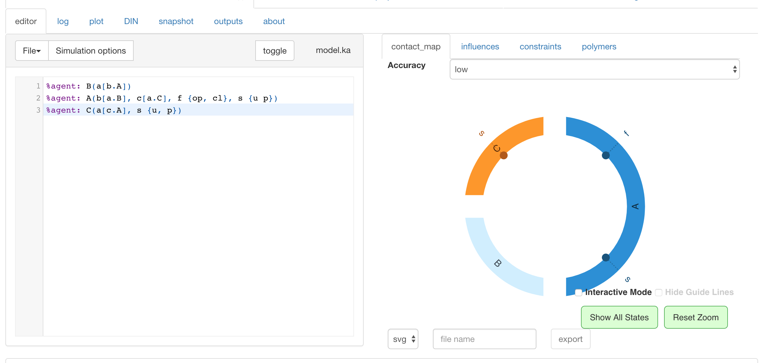
cf. pictures
Steady state of the system strongly biased toward “$A$ binds to $B$”: initially,
-
there are
- $N_A × N_B$ patterns of the form $A, B$
- $0$ pattern of the form $A - B$
-
after one binding, there are
- $(N_A-1) × (N_B-1)$ patterns of the form $A, B$
- $1$ pattern of the form $A - B$
⟹ strong biais towards creating bindings, as the rates are all the same
Product inhibition:
\[A+B \leftrightarrow AB ⟶ A^\ast B \leftrightarrow A^\ast + B\\\]⟶ inefficient enzyme
Efficient enzyme:
\[A+B \leftrightarrow AB ⟶ A^\ast B ⟶ A^\ast + B\\\]At home: try $A \text{ phosphorylated}$ ⟹ $A \text{ open}$, and then only $A \text{ open}$ phosphorylates $C$
Stochastic strategies
Petri nets ≃ multi-set rewriting
For example:
\[S, S, T ⟶ S, T, U\]But usually, written with
- Tokens: numbers of symbols $S, T, …$
- Thick lines: rules
In the literature:
- stochastic: probabilities not given, derived from the structure
- probabilistic: probabilities are given
Two things to compute:
- which reaction should trigger? $ℙ_R, ℙ_S, …$
- how long do I have to wait in order to see something happen? ⟹ compute the $dt$ increment
Monte-Carlo simulations: stochastic strategies developed to simulate these systems (invented for the Manhattan project):
- select two tokens at random and see if they can trigger a reaction
⟹ highly inefficient: times it takes to see when something happen depends on the CPU
but better: Gillespie’s algorithm (he’s a physicist) (1970’s) ⟶ introduced an algorithm that was standard in physics and became famous in the biology community
- what is the proba that $R$ triggers versus $S$?
- how long do you have to wait before a rule is triggered?
Which reaction should trigger?
Activity of the system:
\[λ_{P_T} = \sum\limits_{ ρ ∈ \lbrace R, S \rbrace } \underbrace{λ_ρ}_{\text{activity of reaction } ρ}\\ λ_R = \vert P_A \vert × \vert P_B \vert × k_S\\ λ_S = \vert P_{AB} \vert × k_S\\ P_ρ = \frac{λ_ρ}{λ_{P_T}}\] \[dt \sim λ_{P_T} \exp(-λ_{P_T} t) \sim \frac 1 {λ_{P_T}}\]Then: from Petri net to Continuous Time Markov Chain (CTMC)
cf. pictures
Leave a comment