$\color{DarkCyan}{τ_u}$ too big: unbind before phosphorylation (too liquid)
$\color{DarkCyan}{τ_u}$ too small: never unbind (too sticky)
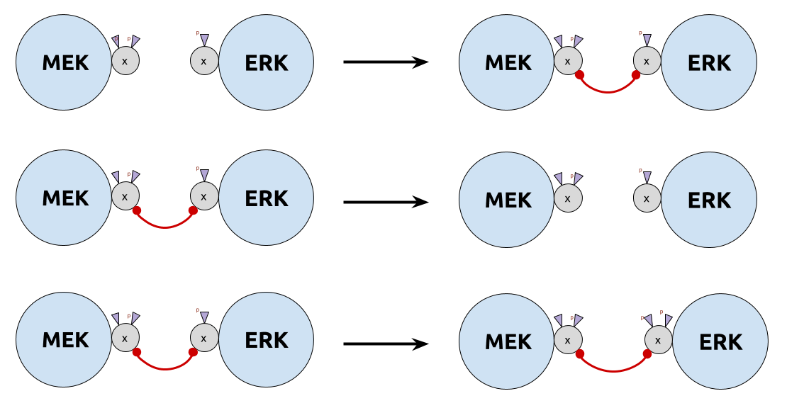
Category of site graphs: $\SGph$
Objects $(V, λ, σ, μ)$:
$V$: set of nodes
$λ: V ⟶ 𝒜$: name assignment
$σ: V ⟶ 𝒫(𝒮)$: site assignment
$μ: \underbrace{\text{ matching}}_{\rlap{\text{irreflexive symmetric binary relation}}}$ over $\sum\limits_{ v ∈ V } σ(v)$
Morphism $f: (V, λ, σ, μ) ⟶ (V', λ', σ', μ')$:
Name/site/edge-preserving and edge reflecting monomorphism $f: V ⟶ V'$
Signature $Σ: 𝒜 ⟶ 𝒮$:
$x ≤ Σ \quad ⟺ \quad σ_x(V_x) ⊆ Σ(λ_x(V_x))$
$Σ ≤ x \quad ⟺ \quad Σ(λ_x(V_x)) ⊆ σ_x(V_x)$
Epimorphisms
Forgetful functor to the category of graphs:
$$U: \SGph ⟶ \Gph$$
Epimorphisms from $x$ to $y$:
$$[x, y]^e \; ≝ \; \big\lbrace h ∈ \underbrace{\Hom[\SGph]{x, y}}_{\text{denoted by } [x,y]} \; \mid \; h \text{ is an epi (i.e. right-cancellable)} \big\rbrace$$
Lemma:
$$h ∈ \overbrace{\Hom[\SGph]{x, y}}^{\text{denoted by } [x,y]} \text{ is an epi } \\ \; ⟺ \; ∀ c_y ⊆ y \text{ connected component}, \, h^{-1}(c_y) ≠ ∅$$
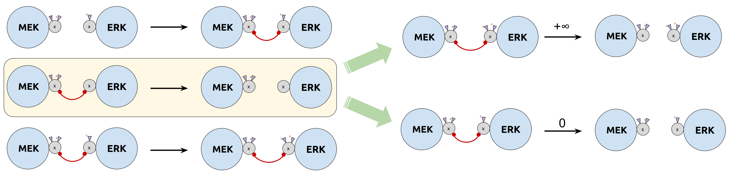
Epi-mono factorisation
Factorisation:
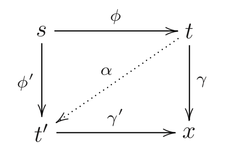
$f ∈ [s, x]$ is said to be factored by $t$ if $f = γ ϕ$ for $ϕ ∈ [s, t]^e$ and $γ ∈ [t, x]$
Every iso $α ∈ [t, t']$conjugates the factorisations $ϕ, γ$ and $ϕ', γ'$:
⟹ Equivalence relation:
$$ϕ, γ \; ≃_{tt'} \; ϕ', γ'$$
The group $[t, t]$ acts freely on $[s, t]^e × [t, x]$ (as we have epis and monos), so by Burnside’s lemma:
V. Danos, J. Feret, W. Fontana, R. Harmer, and J. Krivine, “Rule-Based
Modelling, Symmetries, Refinements,” in Formal Methods in Systems
Biology, vol. 5054, J. Fisher, Ed. Berlin, Heidelberg: Springer Berlin
Heidelberg, 2008, pp. 103–122.
E. Murphy, V. Danos, J. Féret, J. Krivine, and R. Harmer, “Rule-Based
Modeling and Model Refinement,” in Elements of Computational Systems
Biology, H. M. Lodhi and S. H. Muggleton, Eds. Hoboken, NJ, USA: John
Wiley & Sons, Inc., 2010, pp. 83–114.
“List of signalling pathways,” Wikipedia. 30-Nov-2016.
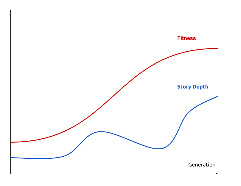
 BUT counter-intuitive
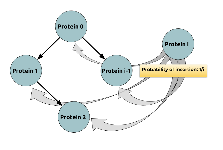 $$ \begin{align*} & 𝔼(\max_i \depth(P_i)) \\ & ≤ 𝔼\Big(\ln\Big(\underbrace{\sum\limits_{ i=0 }^n \exp(\depth(P_i))}_{\; ≝ \; α_n}\Big)\Big) \\ & ≤ \ln \underbrace{𝔼(α_n)}_{\rlap{\substack{= \; 𝔼(α_{n-1}) + 𝔼(\exp(\depth(P_n))) \\ = \, (1 + \frac e i) \, 𝔼(α_{n-1})}}}\\ & = \ln \Big(\prod\limits_{ i=1 }^n \Big(\underbrace{1 + \frac e i}_{≤\, \exp (\frac e i)}\Big) \Big) = e H_n \sim \boxed{e \ln n} \end{align*} $$