[Project] Coherent Patterns of Activity from Chaotic Neural Networks
AT2 – Final Project: Coherent Patterns of Activity from Chaotic Neural Networks
Younesse Kaddar
From “Generating Coherent Patterns of Activity from Chaotic Neural Networks” by D. Sussillo and L.F.Abbott (2009)
| iPython notebook | Documentation | Github | Report | |
|---|---|---|---|---|
1. Networks Architectures
We will consider (sparse) recurrent neural networks of $N_G$ neurons, that can be thought of as simple models actual biological neural networks:
-
the neurons are inter-connected by synapses (which may be excitatory or inhibitory)
-
each neuron’s membrane potential follows a leaky integrate-and-fire-looking differential equation (which depends network architecture details)
-
the network is a linear combination of the neurons’ activites weighted by readout vector(s) (the latter will be modified during the learning process)
-
there may be external inputs and/or the network output may be fed back to the network (directly or via a feedback network).
Network Architecture A
The first network architecture is the following recurrent generator network:
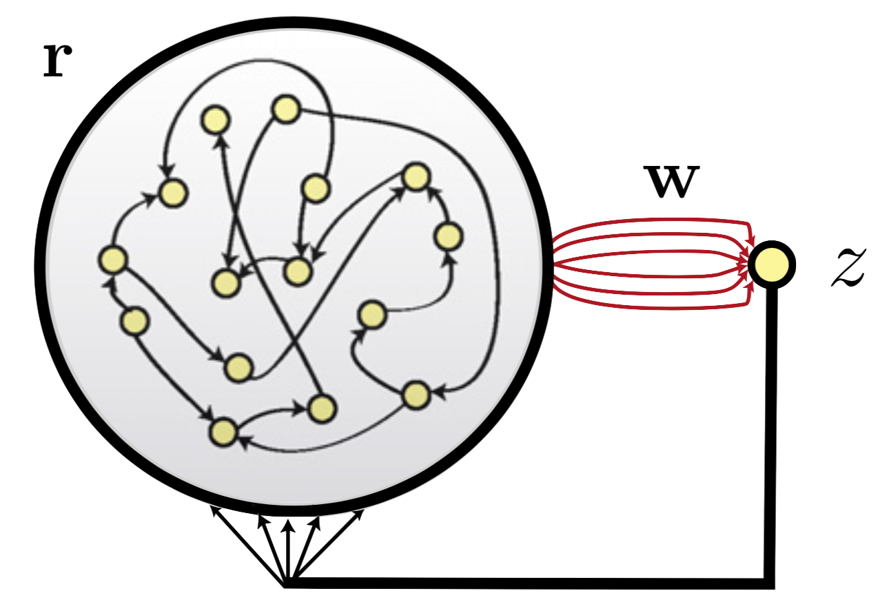
where
- the large cicled network is the generator network
- $\mathbb{r}$ is the neurons’ firing rates
- $\mathbb{w}$ is the readout vector: its weights are only ones prone to be modified during training (indicated by the red color, contrary to the black connections, that remain unchanged thoughout learning)
The only feedback provided to the generator network comes from the the readout unit.
Here, the membrane potential of neuron $i ∈ [1, N_G]$ is given by:
\[τ \dot{x}_i = -x_i + g_{GG} \sum\limits_{j=1}^{N_G} J_{ij}^{GG} \underbrace{\tanh(x_j)}_{≝ \, r_j} + g_{G_z} J_i^{G_z} z\]- $x_i$ is the neuron’s membrane potential
-
$τ = 10 \text{ ms}$ is the time constant of the units dynamics
- $J^{GG}$ is the synaptic weight/strength matrix of the generator network
-
$g_{GG}$ is the scaling factor of the synaptic weight matrix of the generator network
- $J^{Gz}$ is the readout unit weight matrix (applied when the readout unit is fed back in the generator network)
- $g_{Gz}$ is the scaling factor of the feedback loop: increasing the feedback connections results in the network chaotic activity allowing the learning process.
When it comes to the implementation:
- Each element of $J^{GG}$ is set to $0$ with probability $1-p_{GG}$. The nonzero elements thereof are drawn from a centered Gaussian distribution with variance $1/p_{GG}$
- The elements of $J^{Gz}$ are drawn from a uniform distribution between $-1$ and $1$
-
Nonzero elements of $\textbf{w}$ are set initially either to zero or to values generated by a centered Gaussian distribution with variance $1/(p_zN)$.
-
The network integration time step $dt$ and the time span between modifications of the readout weights $Δt$ may not be equal:
\[Δt ≥ dt\]
2. First-Order Reduced and Controlled Error (FORCE) algorithm
Sussilo and Abott’s FORCE supervised learning algorithm makes it possible for chaotic recurrent network output to match a large array of pre-determined activity patterns.
It is different from other classic learning algorithms in that, instead of trying to nullify the error as qickly as possible, it:
- reduces the output error drastically right away
- but then keeps maintaining it small (instead of nullifying it), and rather focuses on decreasing the number of modifications needed to keep the error small
Feeding back an output close but different to the desired one has the following advantages, among others:
-
it avoids over-fitting and stability issues (indeed, and over-fitted chaotic nework may have its activity diverge as soon as a non-zero error is fed back), making the whole procedure suited for chaotic neural networks, which are highly intersting, insofar as many models of spontaneously active neural circuits exhibit chaotic behaviors.
-
it enable us to modify synaptic strength without restricting ourselves to specific neurons (like ouput ones), which makes it all the more realistic, from a biological standpoint.
How and why does FORCE learning work?
How?
We initialize a matrix $P(t)$ - the estimate of the inverse of the network rates correlation matrix plus a regularization term - as follows:
\[P(0) = \frac 1 α \textbf{I}\]where $α$ is the inverse of a learning rate: so a sensible value of $α$
- depends on the target function
- ought to be chosen such that $α « N$
Indeed:
- if $α$ is too small, the learning is so fast it can cause unstability issues
- if $α$ is too large, the learning is so slow that it may end up failing
Then, at each time-step $Δt$:
- \[P(t) ⟵ \Bigg(\textbf{I} - \frac{1}{1+⟨\textbf{r}(t), P(t-Δt)\textbf{r}(t)⟩} \underbrace{P(t-Δt)\textbf{r}(t)\textbf{r}(t)^\T}_{\text{outer product}}\Bigg) P(t-Δt)\]
-
One compute the error before the readout vector update:
\[e_-(t) = \textbf{w}(t-Δt)^\T \textbf{r}(t) - f(t)\] -
The readout vector is updated:
\[\textbf{w}(t) ⟵ \textbf{w}(t-Δt) - e_-(t) P(t) \textbf{r}(t)\]
If $α « N_G$, then it can be shown that the error is remains small from the first update on, and $\textbf{w}$ converges to a constant value, all thoughout $P$ converging toward the pseudo-inverse of $\sum\limits_{ t } \textbf{r}(t)\textbf{r}(t)^\T + \frac 1 α \textbf{I}$ and the error being reduced.
Why?
Essentially, FORCE relies on a regularized version of the recursive least-squares (RLS) algorithm (that is, the online/incremental verison of the well-known least-squares algorithm).
Basically, what one attempts to do is an online regression (but with the contraints mentioned above), where we try to find a predictor $\hat{f}$ such that:
\[f(t) = \hat{f}(\textbf{x}(t))\]of the form
\[\hat{f}(\textbf{x}(t)) = \sum\limits_{ i=1 }^{N_G} \tanh(\textbf{x}_i(t)) \textbf{w}_i = ⟨ \underbrace{\tanh(\textbf{x}(t))}_{ =\, \textbf{r}(t)} , \textbf{w}⟩\]So in a batch fashion, where we consider several observations for several consecutive timesteps (the $\textbf{r}(t)$ are the lines of a matrix $\textbf{R} = \tanh(\textbf{X})$):
\[\hat{f}(\textbf{X}) = \tanh(\textbf{X}) \textbf{w}\]In an online fashion: at each step $t$, one has the input/desired output pair:
\[\big(\textbf{x}(t),\; f(t)\big)\]The squared prediction error thereof is:
\[e_-(t) = \Big(f(t) - \underbrace{\tanh(\textbf{x}(t+1))^\T \textbf{w}(t-Δt)}_{= \, ⟨\textbf{r}(t+1), \textbf{w}(t-Δt)⟩}\Big)^2\]In a batch way, given $n$ input/desired output pairs:
\[\big(\textbf{x}(t),\; f(t)\big), \ldots, \big(\textbf{x}(t+(n-1)Δt),\; f(t+(n-1)Δt)\big)\]the squared error is (where $\textbf{t} ≝ (t, t+Δt, ⋯, t+(n-1)Δt)^\T$):
\[e_{batch} = \frac 1 {2n} \Vert f(\textbf{t}) - \hat{f}(\textbf{X})\Vert_2^2 = \frac 1 {2n} \Vert f(\textbf{t}) - \textbf{R} \textbf{w} \Vert_2^2\\ = \frac 1 {2n} \sum\limits_{ i=0 }^n \Big(f(t+iΔt) - ⟨\textbf{r}(t+iΔt), \textbf{w}⟩\Big)^2\]It is convex with respect to $\textbf{w}$, so to minimize it we set the gradient to zero:
\[\textbf{0} = \nabla_\textbf{w} e_{batch} = - \frac 1 n \sum\limits_{ i=1 }^n \textbf{r}(t+iΔt) \Big(f(t+iΔt) - ⟨\textbf{r}(t+iΔt), \textbf{w}^\ast⟩\Big)\]i.e.
\[\underbrace{\left(\sum\limits_{ i=1 }^n \textbf{r}(t+iΔt) \textbf{r}(t+iΔt)^\T \right)}_{≝ \; A} \; \textbf{w}^\ast = \underbrace{\sum\limits_{ i=1 }^N \textbf{r}(t+iΔt)f(t+iΔt)}_{≝ \; b}\]Therefore:
\[\textbf{w}^\ast = A^\sharp b\]where $A^\sharp$ is the pseudo-inverse of $A$.
So we are beginning to see where this $(A + \frac 1 α \textbf{I})^\sharp$ comes from, in the FORCE algorithm.
It’s even more blatant in the online version of the least squares algorithm: we see that $A$ and $b$ can be computed incrementally at each time-iteration:
\[A(t+Δt) = A(t) + \textbf{r}(t+Δt) \textbf{r}(t+Δt)^\T\\ b(t+Δt)= b(t) + \textbf{r}(t+Δt) f(t+Δt)\]Then, $\textbf{w}^\ast$ can be estimated as:
\[\textbf{w}(t+Δt) = \big(A^{(t+Δt)}\big)^\sharp \; b^{(t+Δt)}\]The key point is that the pseudo-inverse $\big(A^{(t+Δt)}\big)^\sharp$ can be estimated with resort to the
Sherman-Morrison lemma (provided $A(0)$ is non-zero, which is what happens in our case):
\[\left(A + \textbf{r}(t+Δt) \textbf{r}(t+Δt)^\T\right)^\sharp = A^\sharp - \frac{A^\sharp \textbf{r}(t+Δt) \textbf{r}(t+Δt)^\T A^\sharp}{1+\textbf{r}(t+Δt)^\T A^\sharp \textbf{r}(t+Δt)}\]
which is what gives $P$’s update-rule.
Implementation and Results
Our implementation makes use of object-oriented programming:
-
it can be found here as a python package
-
to import it with
pip:!pip install git+https://github.com/youqad/Chaotic_Neural_Networks.git#egg=chaotic_neural_networks from chaotic_neural_networks import utils, networkA
-
-
the documentation is here
The package structure is as follows:
Chaotic_Neural_Networks
│
└───chaotic_neural_networks
│   │   __init__.py
│   │   utils.py
│   │   networkA.py
│
└───docs
    │   ...
utils.pycontains utility functions, among which target function such as a sum of sinusoids, a triangle-wave, etc…-
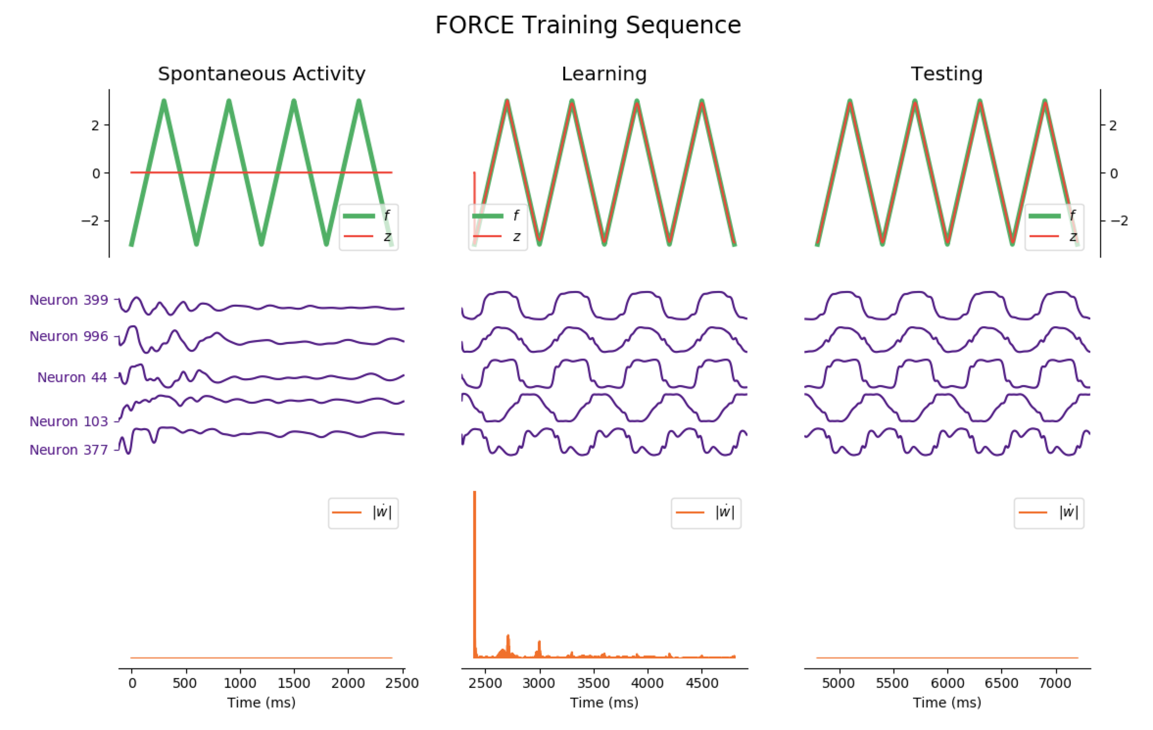
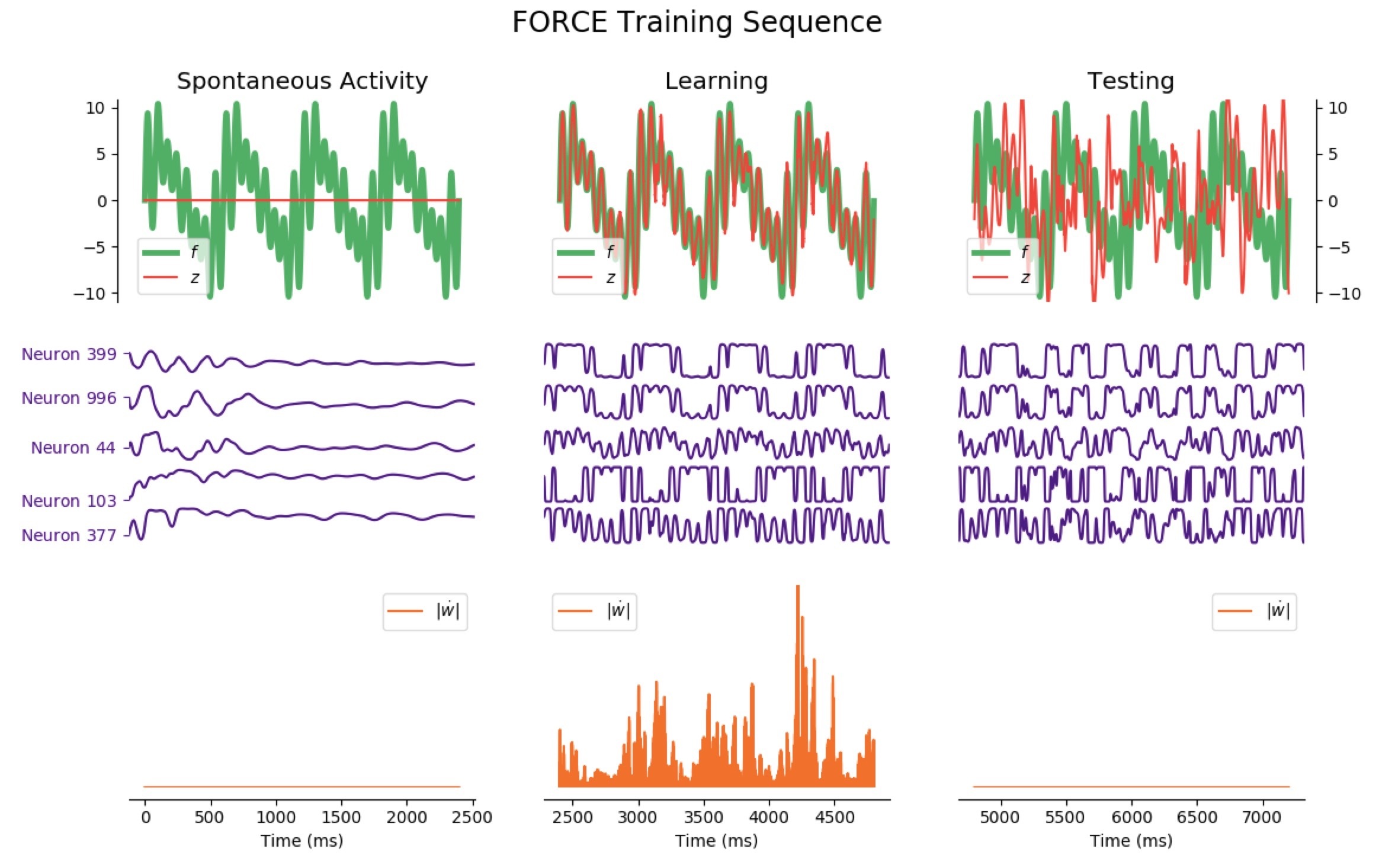
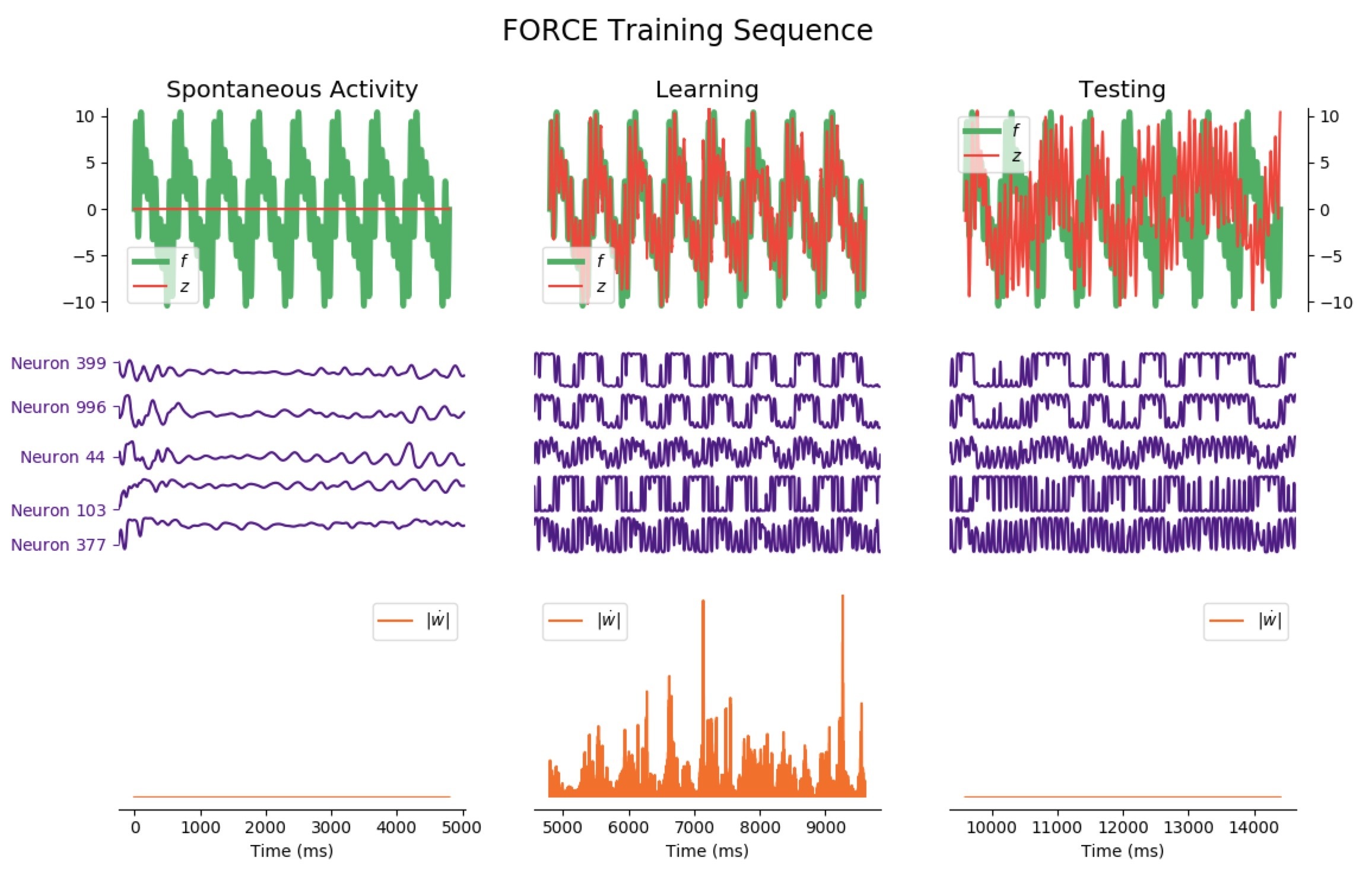
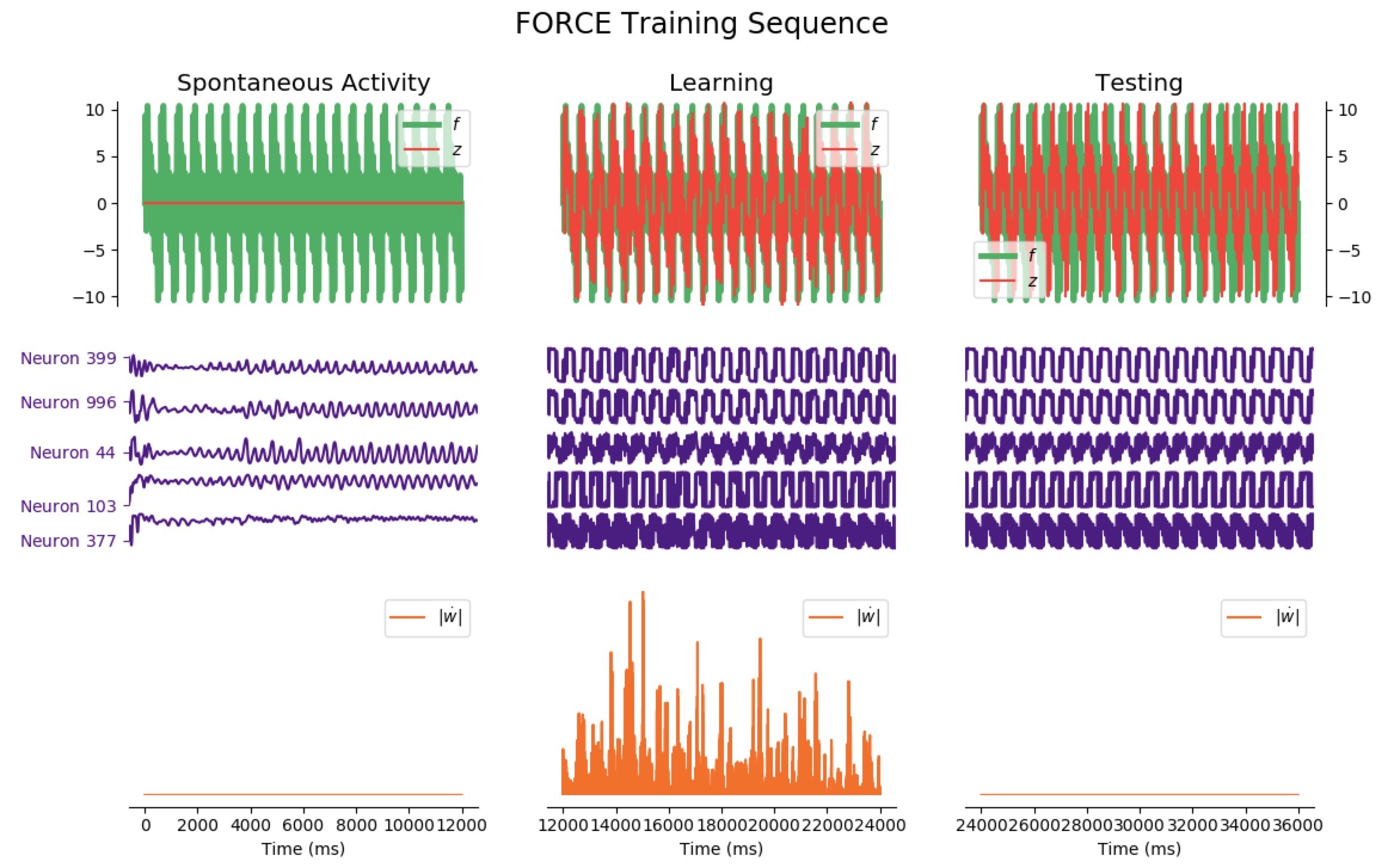
networkA.pyis the module related to the first architecture: the classNetworkAis a way to instantiate such a network (which can be fully parametrized with the optional arguments). The three most important methods are:errorwhich computes the average train/test error of the networkstep, which executes one step of lengthdtof the network dynamicsFORCE_sequence, which plots (returns a matplotlib figure to be precise) a full training sequence of the FORCE algorithm: showing the evolution of the network ouput(s), a handful of neurons membrane potential, and the time-derivative of the readout vector $\dot{\textbf{w}}$ before training (spontaneous activity), throughout training, and after training (test phase).
For instance: the following code
import matplotlib.pyplot as plt
from chaotic_neural_networks import utils, networkA

t_max = 2400 # in ms: duration of each phase (pre-training, training, and test)

# Target function f: Sum of sinusoids
network1 = networkA.NetworkA(f=utils.periodic)

network1.FORCE_sequence(2400*3)

plt.show()
outputs:
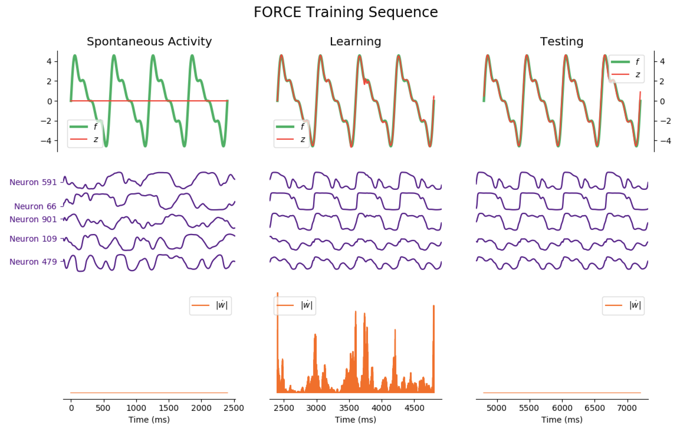
The code to generate the following training sequence plots is in the training_sequence_plots.py file of the github repository (here).
Average Train Error: $0.016$ Average Test Error: $0.055$
Considering the decrease of $\vert \dot{\textbf{w}} \vert$, we see that the learning process is far quicker for the triangle-wave function than for the sum-of-sinusoids one (which is not surprising, as the triangle-wave is piecewise linear): for the former, it takes between 3 and 4 periods for the learning to be complete.
Here are animated gifs of the FORCE learning phase for these target functions (the code to generate these animations is in the Jupyter notebook, the function used is utils.animation_training):
-
Evolution of FORCE learning for a sum of four sinusoids as target:
-
Evolution of FORCE learning for triangle-wave as target:
Now, let us investigate more complicated patterns: we reiterate the FORCE learning procedure, but this time for a significantly more complicated target:
Average Train Error: $0.725$ Average Test Error: $5.730$
Average Train Error: $0.880$ Average Test Error: $5.789$
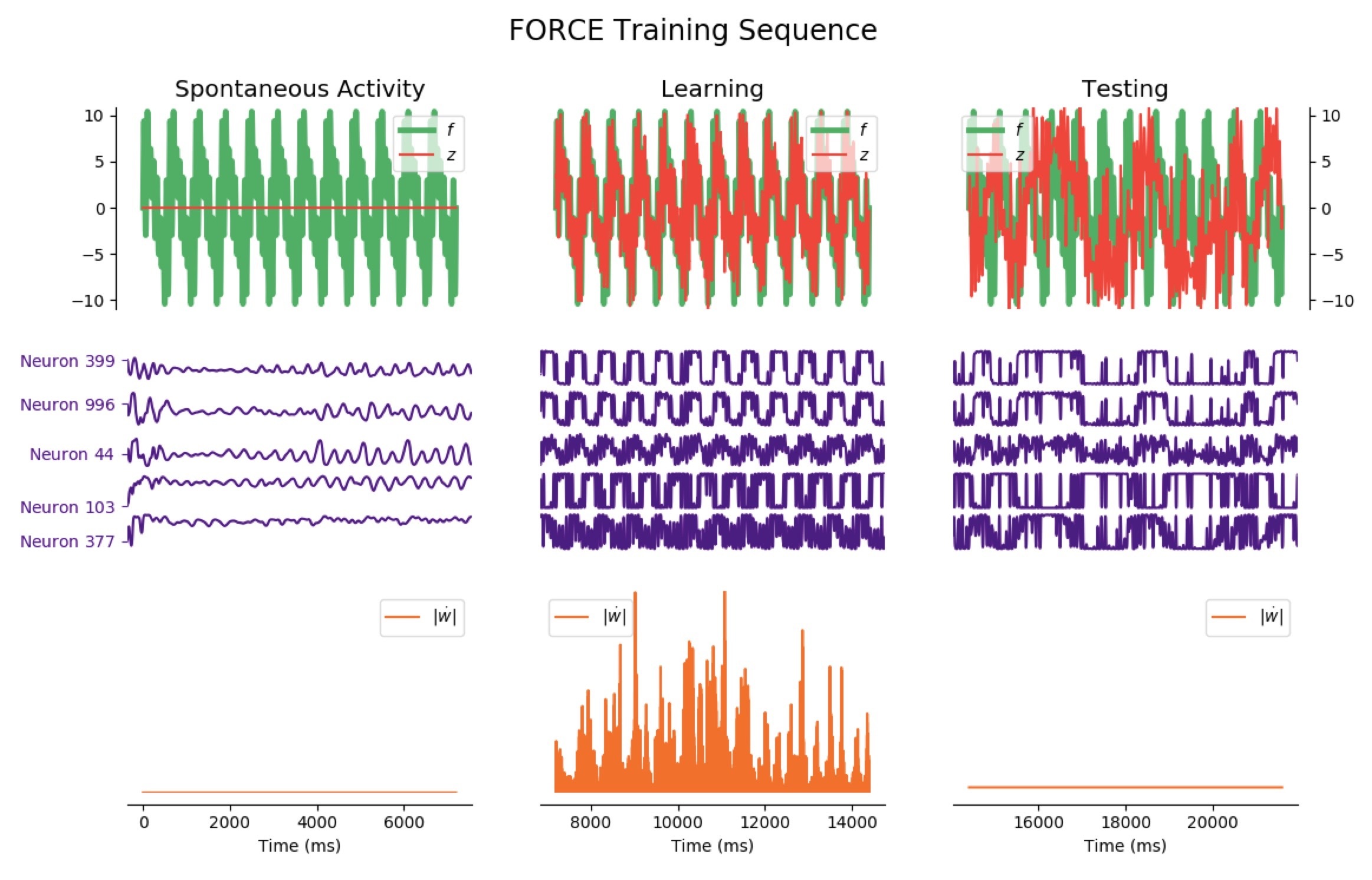
Average Train Error: $0.934$ Average Test Error: $5.993$
Average Train Error: $0.893$ Average Test Error: $5.887$
It appears that the high variability of this target makes matters more complicated: when it comes to learning, the network is still reasonably effective right away, but it has poor testing accuracy for phases lasting less than 12 seconds (the train and test errors even increase until 7 seconds, and then decreases for longer phases).
The network may also have several outputs, corresponding to several readout units. Here are some instances of 2 and 3 output networks:
Two simultaneous outputs
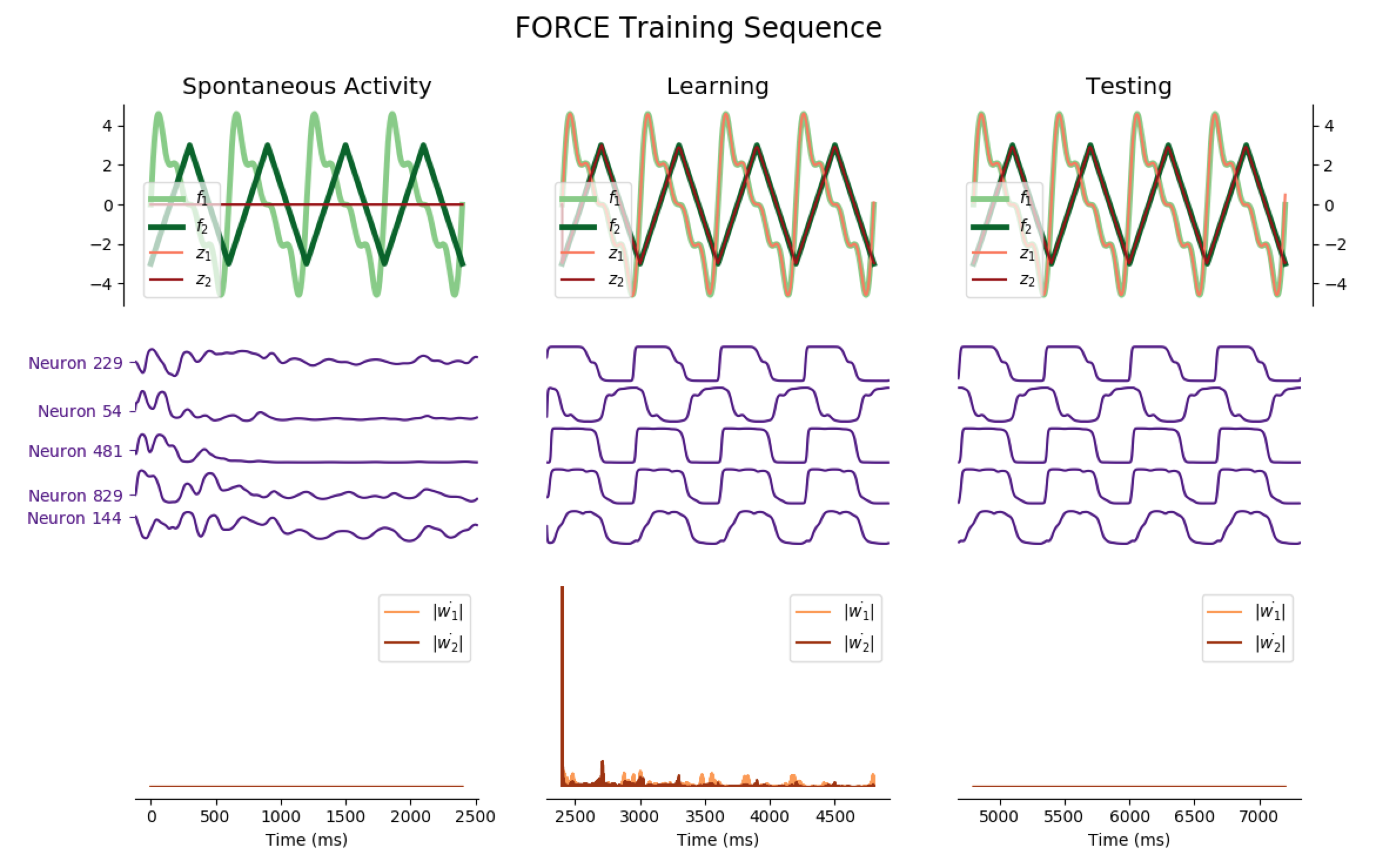
Average Train Errors: $(0.017, 0.010)$ Average Test Errors: $(0.067, 0.040)$
Three simultaneous outputs
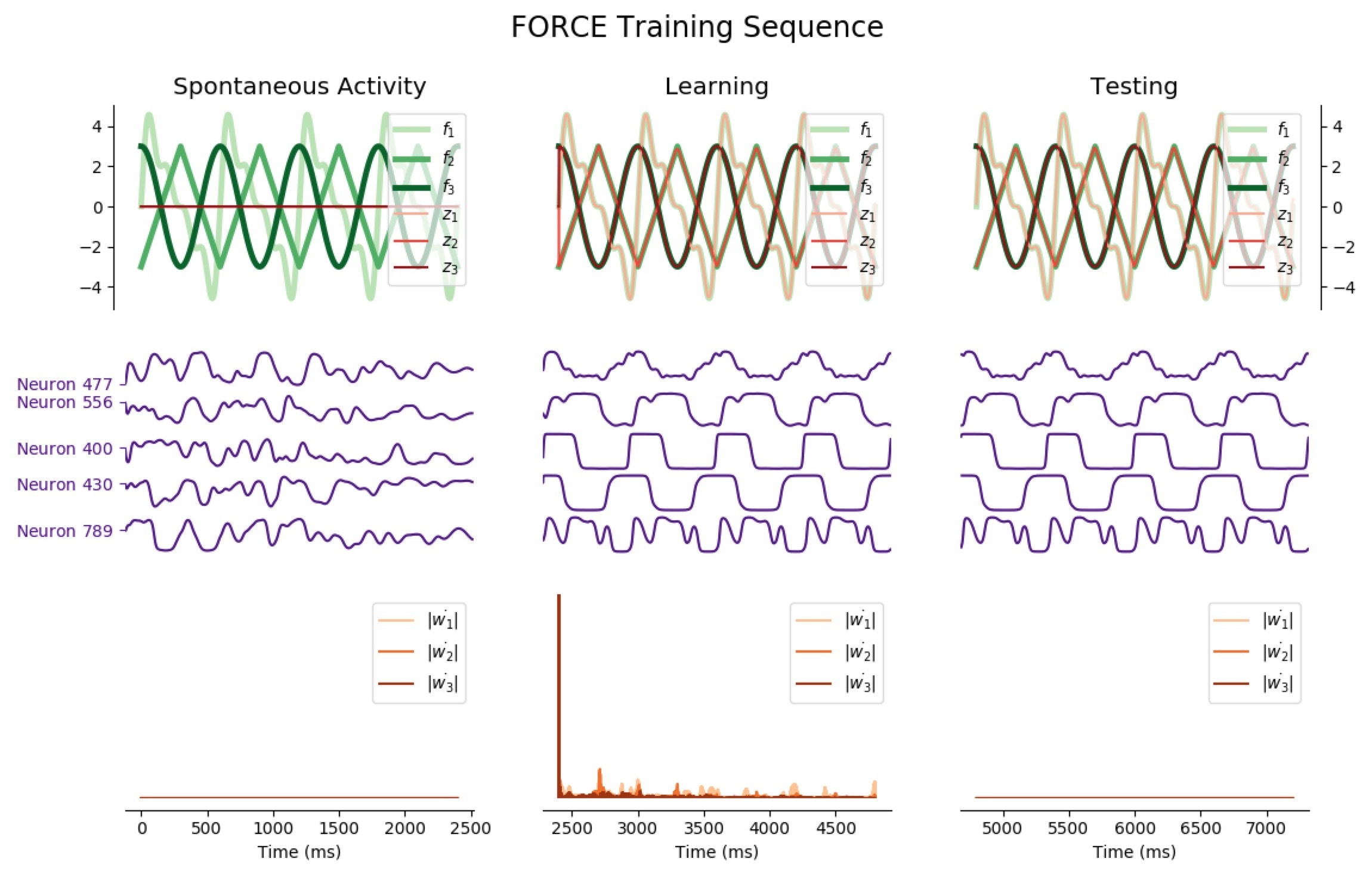
Average Train Errors: $(0.019, 0.012, 0.009)$ Average Test Errors: $(0.073, 0.050, 0.050)$
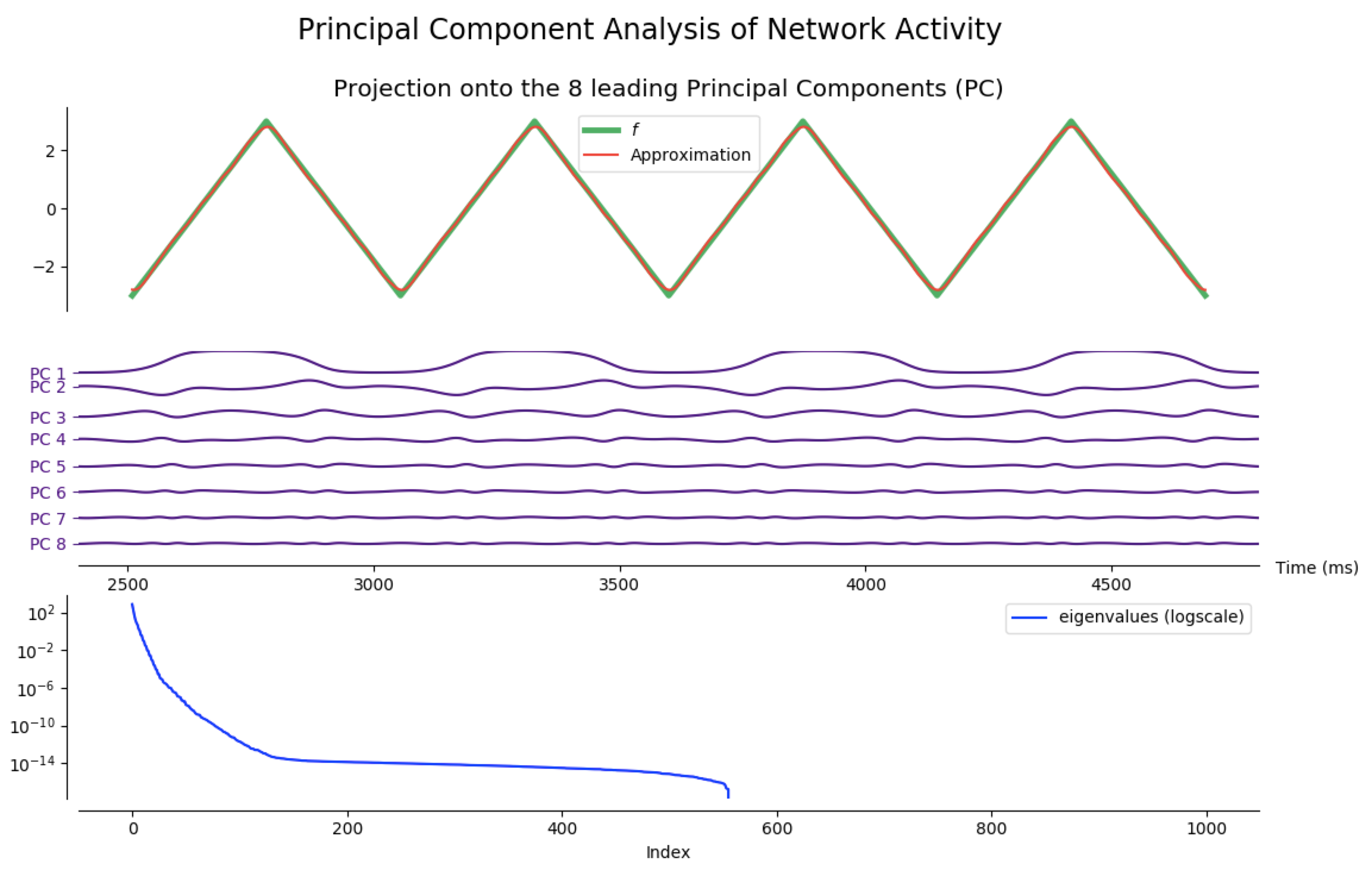
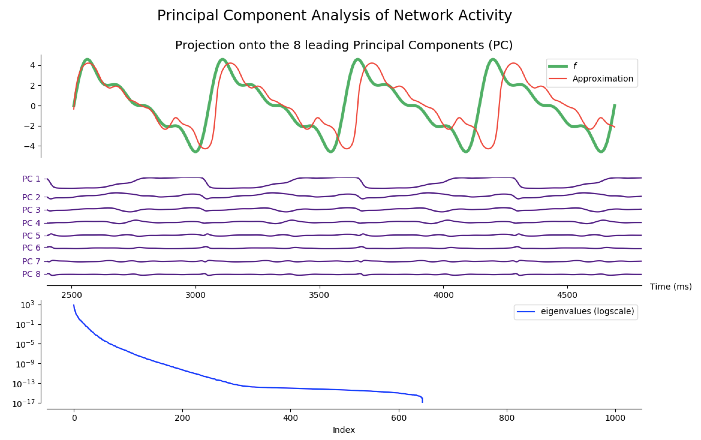
Principal Component Analysis (PCA)
As a matter of fact, most of the network activity can be accounted for by a few leading principal components.
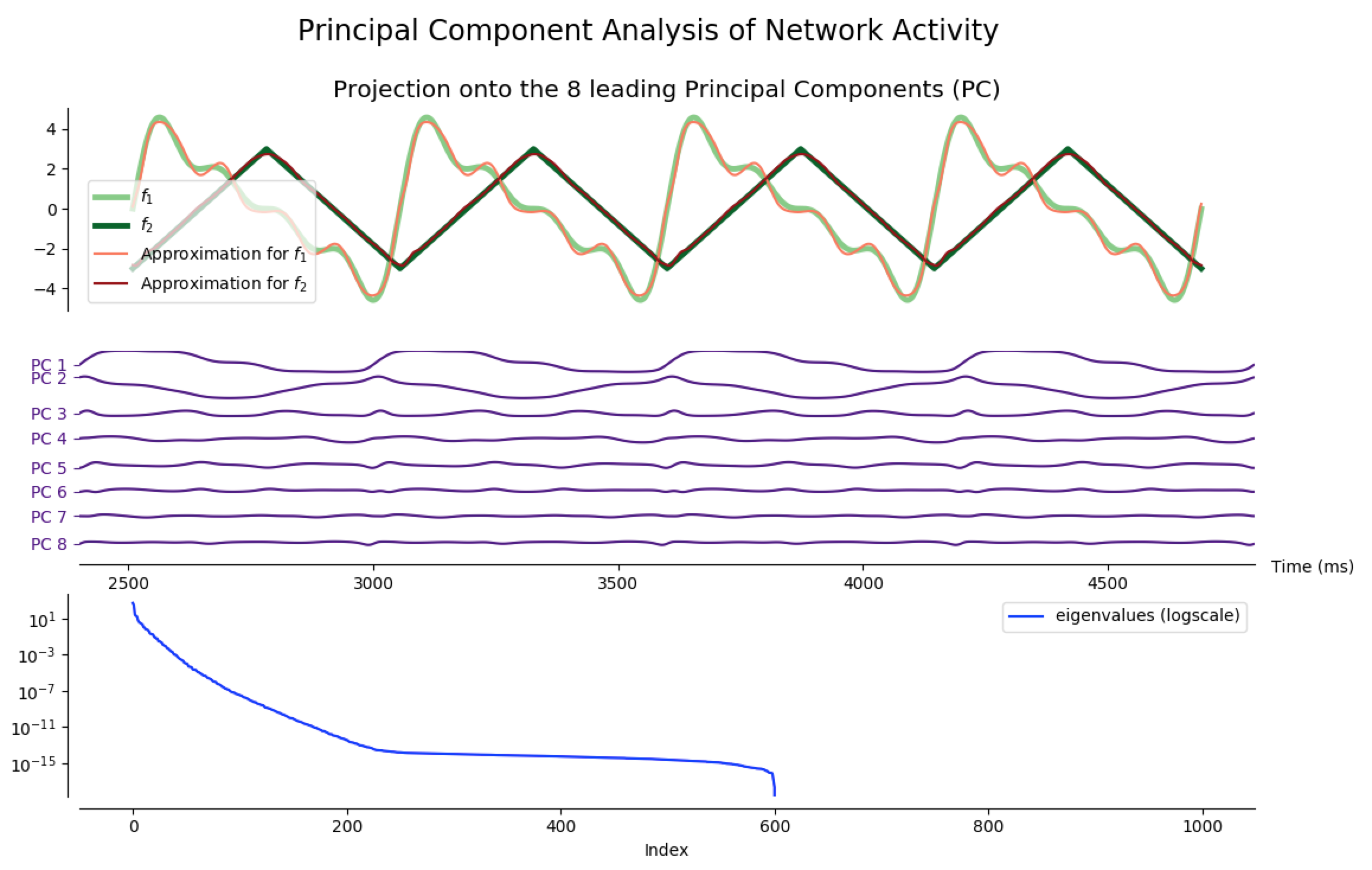
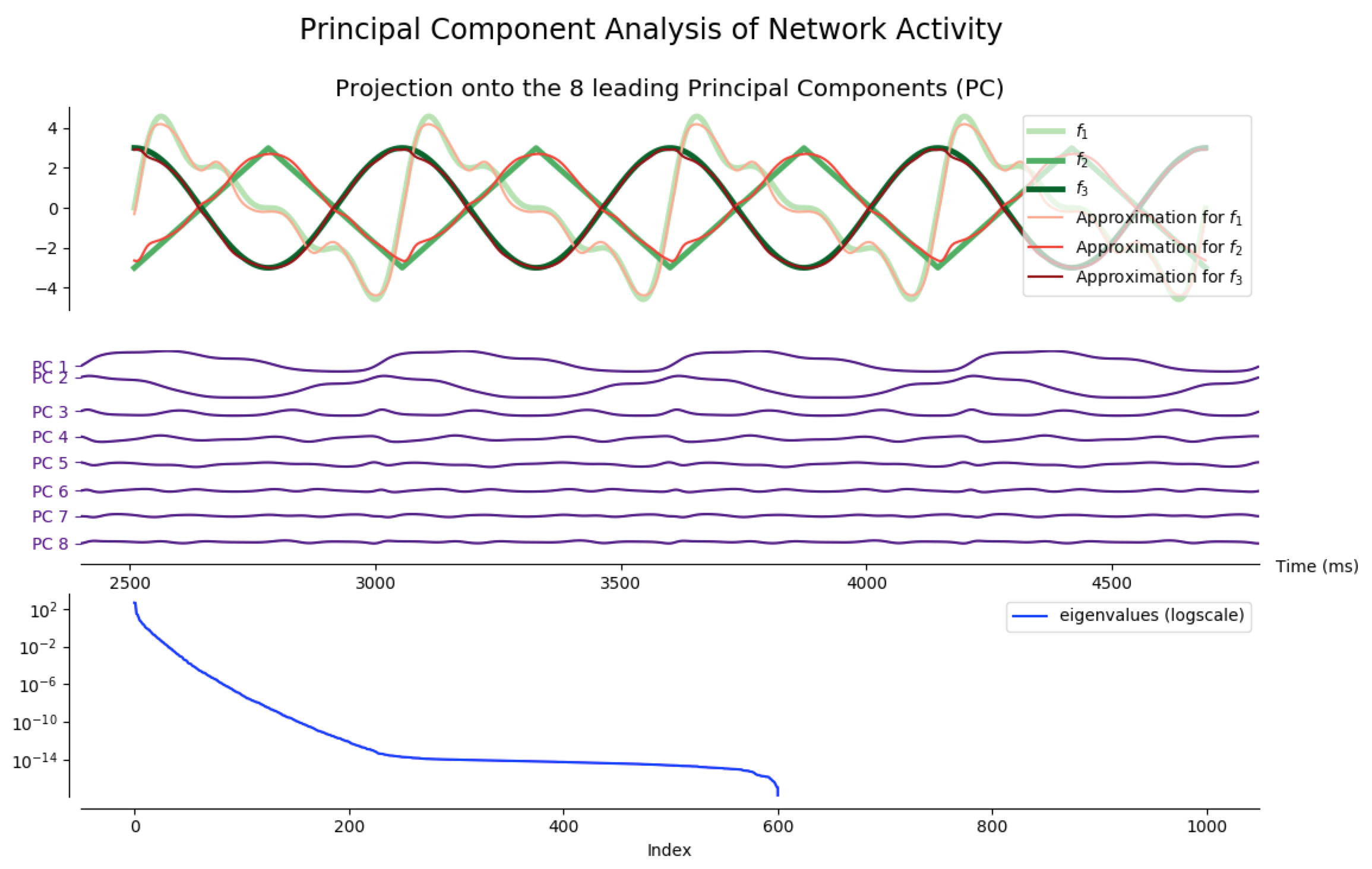
Indeed, after training the network so that it produces different target functions (for various numbers of outputs), one can apply principal component analysis (PCA) to project the network activity on a handful (8 is enough for the following examples) of principal components. Then, it appears that most of the target patterns can be obtained from these few projections: out the hundreds of degrees of freedom available (one thousand in our case, as $N_G=1000$), only a dozens are actually necessary to produce the target functions we have considered.
NB: the code to generate the following figures is in the principal_component_plots.py file of the github repository.
Leave a comment