[Problem Set 2 Quantitative models of behavior] Problem 3: The drift diffusion model of decision-making
Link of the iPython notebook for the code
AT2 – Neuromodeling: Problem set #2 QUANTITATIVE MODELS OF BEHAVIOR
PROBLEM 3: The drift diffusion model of decision-making.
We consider a two-alternative forced choice task (2AFC-task): the subject (e.g. a monkey) sees a cluster of moving dots (in many directions) on a screen and is to choose (whenever he/she/it wants) whether they are moving upwards or downwards.
In the drift-diffusion-model, the subject is assumed to compare two firing rates:
- one firing rate of an upward-motion sensitive neuron, denoted by $m_A$
- and another one from a downward-motion sensitive neuron, denoted by $m_B$
Then, the subjects integrates the difference as follows:
\[\dot{x} = m_A − m_B + σ η(t)\]where $η(t) \sim 𝒩(0, 1)$ is a Gaussian white noise.
For a given threshold $μ$:
- if $x ≥ μ$ then the subject chooses $A$
- else if $x ≤ -μ$ then the subject chooses $B$
We have the following discrete approximation of the drift-diffusion-model:
\[x(t+∆t) = x(t) + (m_A - m_B) ∆t + σ η(t) \sqrt{∆t}\]1. Reaction times
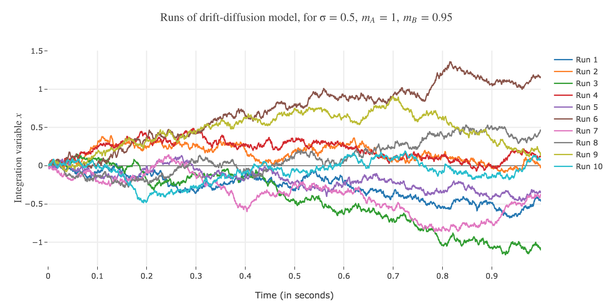
Let $m_A ≝ 1, m_B ≝ 0.95, \, σ ≝ 0.5, \, x(0) ≝ 0$, and $∆t ≝ 0.1 \, \mathrm{ ms}$.
Let us run the drift-diffusion-model ten times with the above parameters, with resort to the Euler method:
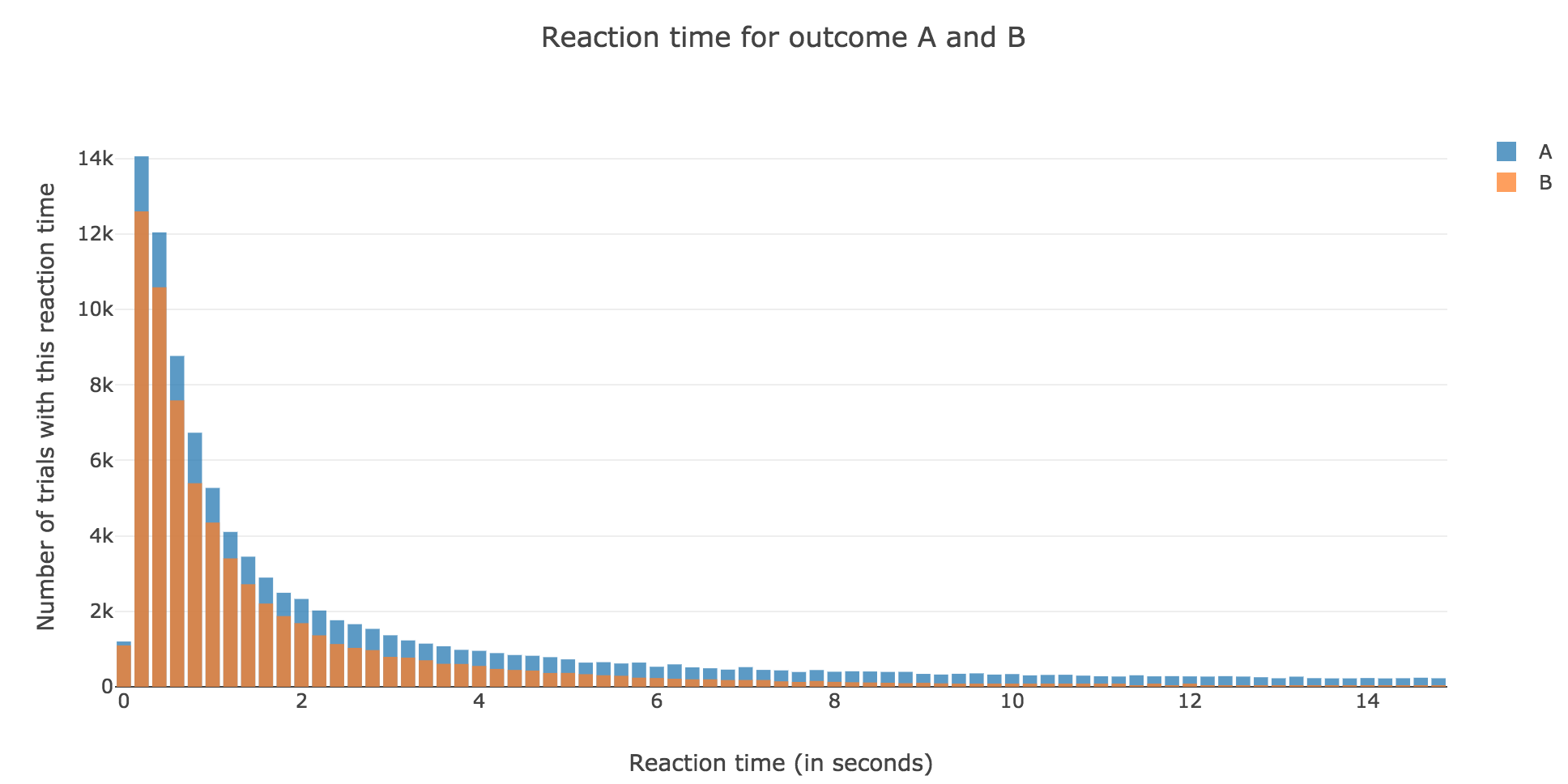
Now, after running the model $N$ times and storing the outcome and the time of threshold crossing (denoted by $t_i$) for each run: let us plot the distribution of reaction times for outcome $A$ and $B$, given that the reaction time is given by:
\[RT_i = 100 + t_i\]-
For $N ≝ 1000$:
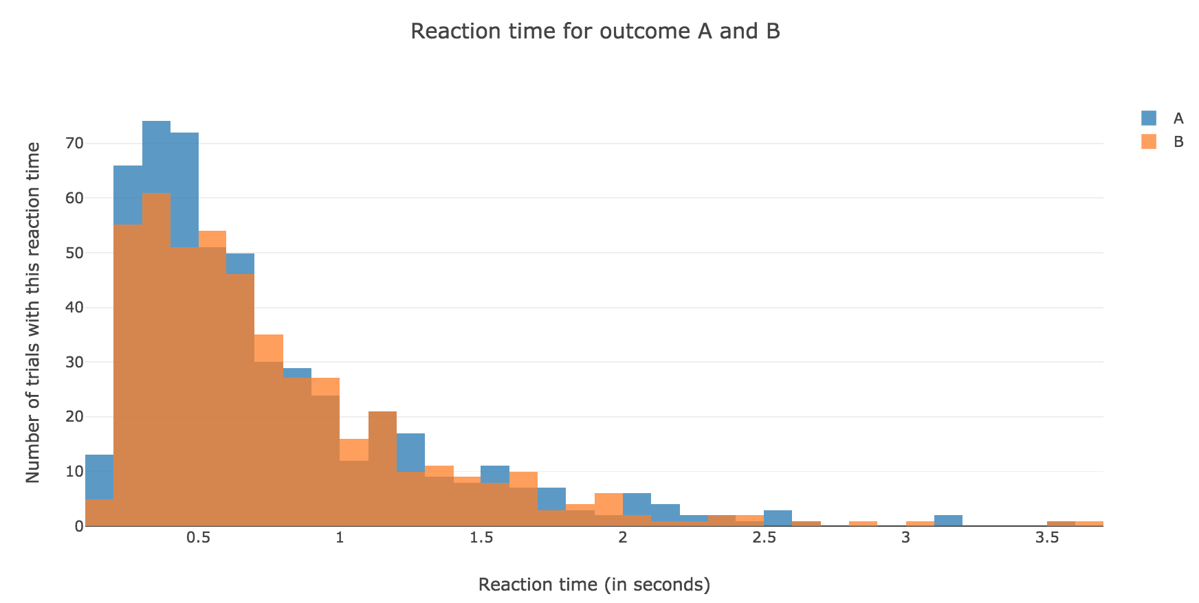
Figure 1.1. - Distribution of reaction times for outcome $A$ and $B$ after running the model $N = 1000$ times -
For $N ≝ 10000$:
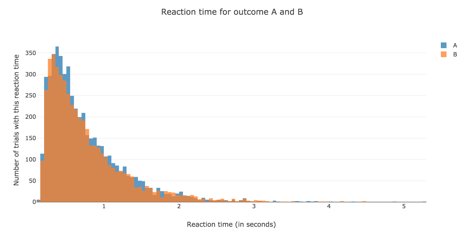
Figure 1.2. - Distribution of reaction times for outcome $A$ and $B$ after running the model $N = 10000$ times
2. Probability of outcome $A$
Let us define the evidence for outcome $A$ versus outcome $B$ as:
\[m_E ≝ m_A - m_B\]The analytical formula of the probability of outcome $A$ is:
\[p_A ≝ \frac{1}{1+ \exp(-β m_E)}\]where $β ≝ \frac{2 μ}{σ^2}$.
Let us compare it, for values of $m_E$ ranging from $-0.2$ to $0.2$, with the empirical probability we can get from our simulation, by running the model $N$ times (for $N$ sufficiently large) and computing:
\[P(A) ≝ \frac{\text{Number of trials of outcome } A}{\text{Number of trials of outcome } A + \text{Number of trials of outcome } B}\]The problem is that we have to compute this empirical probability for several values of $m_E$ ranging from $-0.2$ to $0.2$! As a matter of fact: the previous naive algorithm, based on the Euler method, is far too slow…
But we can cope with that with a trick!
Fast algorithm to compute the distribution of reaction times
From the discrete approximation of the drift-diffusion-model:
\[x(t+∆t) = x(t) + m_E ∆t + σ η(t) \sqrt{∆t}\]So for all $n ≥ 1$:
\[x(t+ n ∆t) = x(0) + n \cdot m_E ∆t + σ \sqrt{∆t} \sum\limits_{ i=1 }^n η_i(t)\]where the
\[η_i(t) \sim 𝒩(\overbrace{0}^{ ≝ \, μ_i}, \overbrace{1}^{≝ \, σ_i^2})\]are independent and normally distributed random variables.
But it is well known that a sum of independent and normally distributed random variables is also a normally distributed variable, such that:
\[\sum\limits_{ i=1 }^n η_i(t) \sim 𝒩\left(\sum\limits_{ i=1 }^n μ_i \, , \; \sum\limits_{ i=1 }^n σ_i^2\right)\]i.e.
\[\sum\limits_{ i=1 }^n η_i(t) \sim 𝒩(0, n)\]But as it happens:
\[\sqrt{n} \underbrace{η(t)}_{\sim 𝒩(0, 1)} \sim 𝒩(0, n)\]So for all $n ≥ 1$, we can set $x(t + n ∆t)$ to be:
\[x(t + n ∆t) = x(0) + n \cdot m_E ∆t + \sqrt{n} \cdot σ \sqrt{∆t} η(t)\]where $η(t) \sim 𝒩(0, 1)$
So solving for $n$ in the threshold crossing conditions:
\[x(t + n ∆t) = ± μ\]is tantamount to:
-
Analysis: solving (for $ξ$, in $ℂ$) two quadratic equations for a given $η(t) ∈ ℝ$:
\[\begin{cases} m_E ∆t \, ξ^2 + σ \sqrt{∆t} η(t) \, ξ + x(0) - μ = 0&&\text{(outcome A)}\\ m_E ∆t \, ξ^2 + σ \sqrt{∆t} η(t) \, ξ + x(0) + μ = 0&&\text{(outcome A)}\\ \end{cases}\] -
Synthesis: keeping only the roots $ξ$ such that $ξ^2 ∈ ℝ_+$, and setting $n ≝ \lceil ξ^2 \rceil$
which gives us a very fast algorithm!
Finally, we can compare the empirical probability of outcome $A$ with the analytical one:
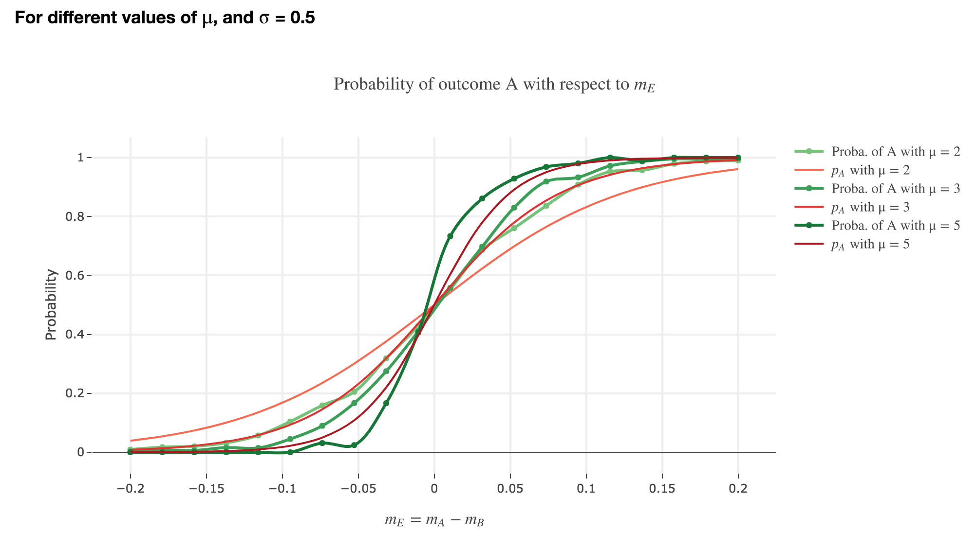
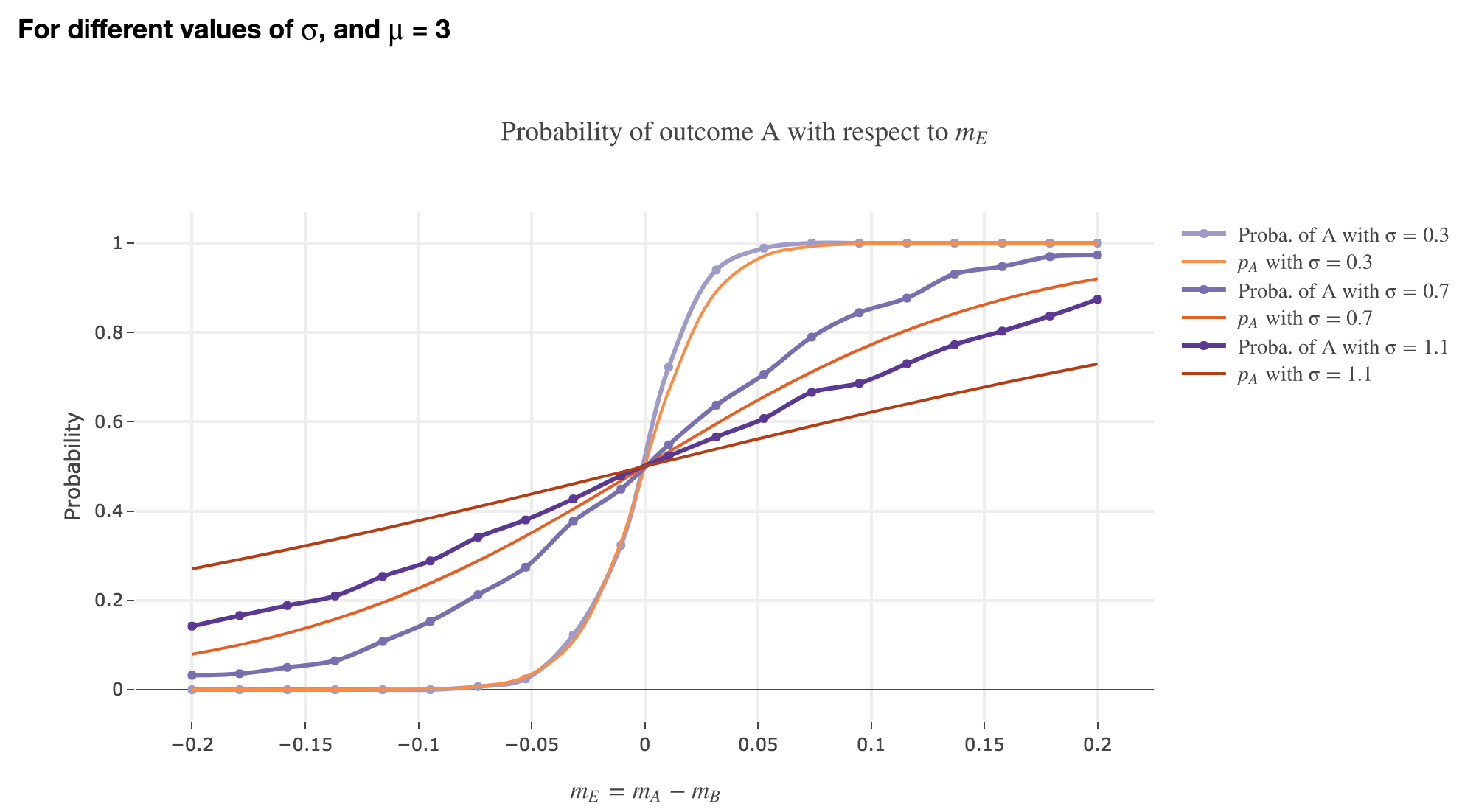
We see that the empirical probability of outcome $A$ matches more and more $p_A$ (when it comes to the shape of the curve):
-
as $μ$ increases
-
as $σ$ decreases (with an almost perfect match above for $σ = 0.3$)
Leave a comment