[Problem Set 2 Quantitative models of behavior] Problem 1: Rescola-Wagner Rule
Link of the iPython notebook for the code
AT2 – Neuromodeling: Problem set #2 QUANTITATIVE MODELS OF BEHAVIOR
PROBLEM 1 - Rescorla-Wagner Model
Let us model a classical conditioning experiment with resort to the Rescorla-Wagner rule.
The experiment is as follows: at trial $i ∈ ℕ$:
- an animal may or may not be presented with a stimulus $u_i$ (e.g.: ringing a bell, clapping hands): $u_i = 1$ if the stimulus is present, $u_i = 0$ otherwise
- … which may or may not in turn be followed by a reward $r_i$ (e.g.: food): $r_i = 1$ if there is a reward, $r_i = 0$ otherwise
The animal is assumed to be willing to predict the correlation between the stimulus and the reward (e.g: by salivating in anticipation): i.e. to predict if it will get the reward based on the presence or absence of the stimulus. As such, the prediction of the animal is denoted by $v_i$ at trial $i$:
\[∀i, \; v_i ≝ w_i u_i\]where $w$ is a parameter learned and updated - trial after trial - by the animal, in accordance with the following Rescola-Wagner rule:
\[w_i → w_i + \underbrace{ε}_{\text{learning rate } << 1} \underbrace{(r_i − v_i)}_{≝ \, δ_i} u_i\]1. Introductory example
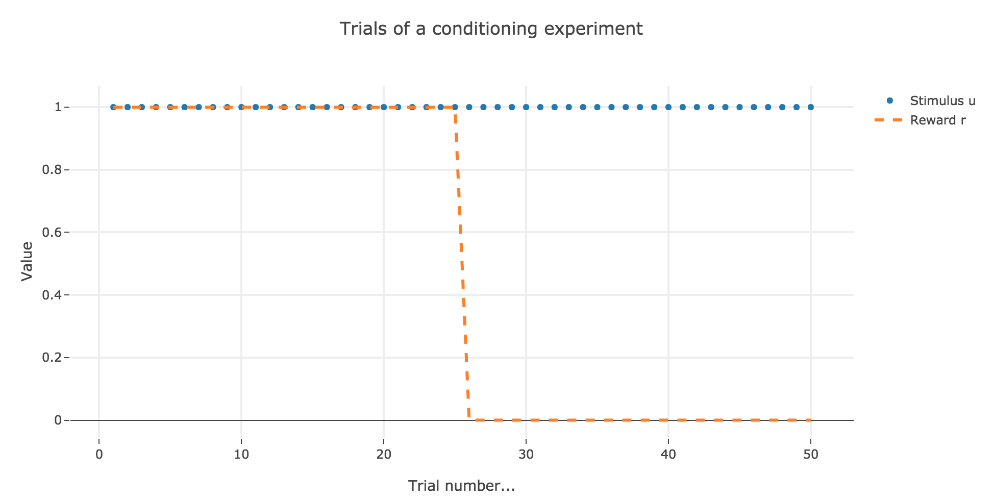
For instance, let us suppose that there are $50$ trials, and:
- during the first $25$ trials, both stimuli and reward are present ($u_i = r_i = 1$)
- during the last $25$ ones, only the stimulus is present ($u_i = 1, \, r_i = 0$)
as illustrated by the following figure:
In which case, according to the Rescola-Wagner rule, the animal prediction $v_i$ is as follows:
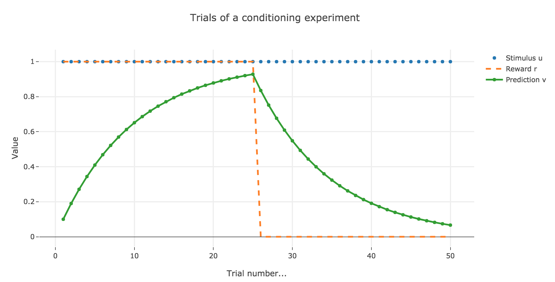
where the learning rate $ε$ is set to be $0.1$.
It appears that the animal prediction $v = wu$ does tend toward the reward. Indeed, if $r_i ≝ r_0$ and $u_i ≝ u_0$ are constant (as it happens here for the first $25$ trials, and for the last $25$ ones):
\[\begin{align*} w_{i+1} & = w_i + ε (r_0 − u_0 w_i) u_0 \\ & = (1- ε u_0^2) w_i + ε r_0 u_0 \\ \end{align*}\]Therefore:
\[\begin{align*} ∀i ≥ i_0, \; w_i &= (1- ε u_0^2)^{i-i_0} \Big(w_{i_0} - \frac{ε r_0 u_0}{1-(1-ε u_0^2)}\Big) + \frac{ε r_0 u_0}{1-(1-ε u_0^2)}\\ &= \frac{r_0}{u_0}\Big(1 - (1-ε u_0^2)^{i-i_0}\Big) + w_{i_0} (1-ε u_0^2)^{i-i_0} \\ \end{align*}\]As a result:
-
for the first $25$ trials: $r_0 = u_0 = 1$ and $w_0 = i_0 = 0$, so that:
\[∀ i ∈ \lbrace 0, 24 \rbrace, \; w_i = 1 - (1-ε)^i \xrightarrow[i \to +∞]{} 1 = r_0\] -
for the last $25$ trials: $r_0 = 0, \; u_0 = 1$ and $i_0 = 24, \, w_{24} > 0$, so that:
\[∀ i ∈ \lbrace 25, 50 \rbrace, \; w_i = w_{24} (1-ε)^{i-24} \xrightarrow[i \to +∞]{} 0 = r_0\]
Changing the learning parameter $ε$
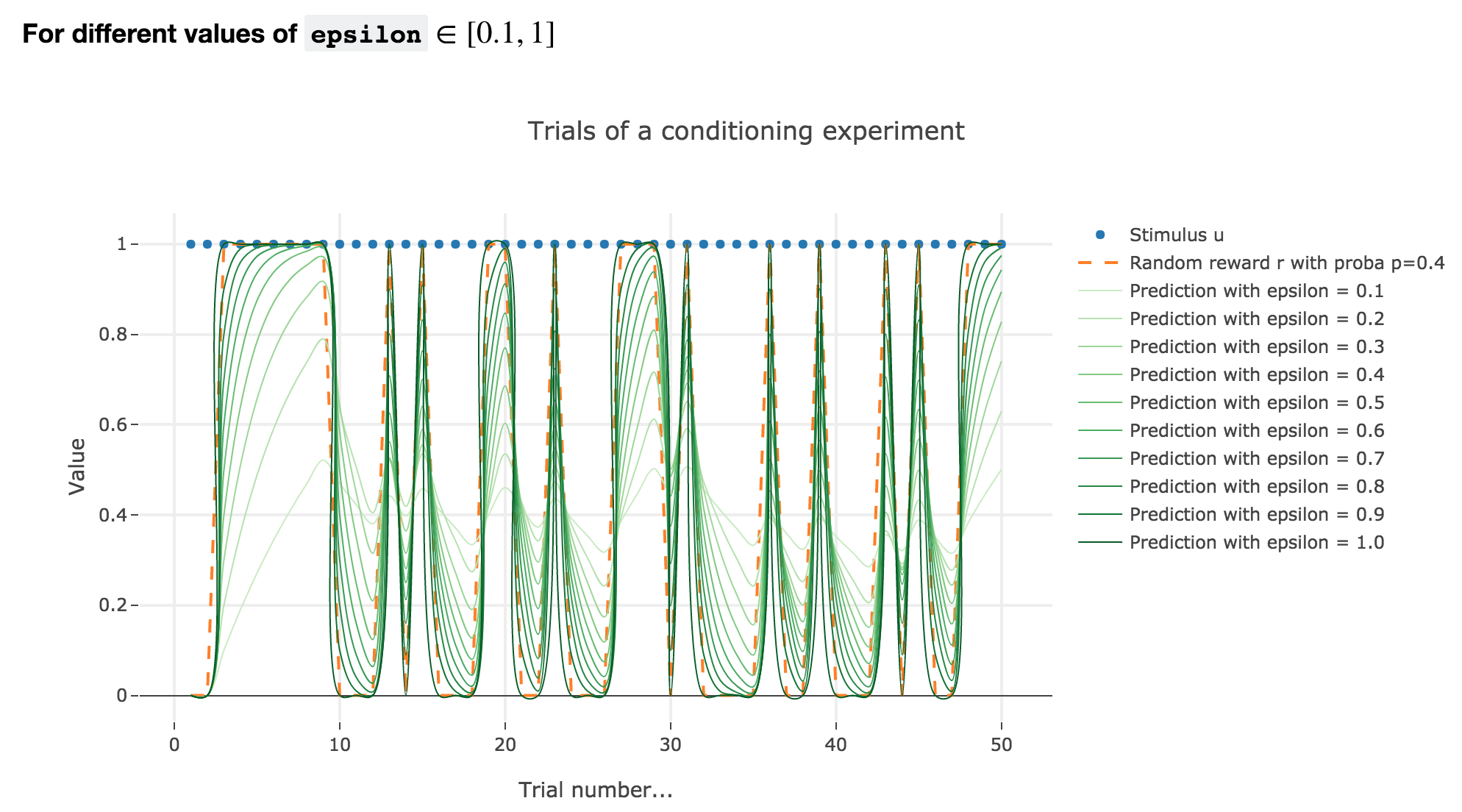
Now, let us change the learning rate $ε$ in the previous example.
For $ε ≤ 1$
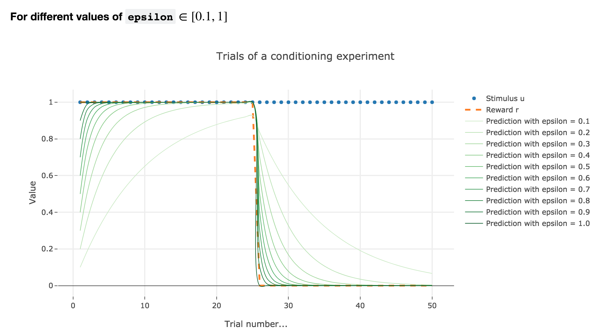
As illustrated by the figure above, when $ε ≤ 1$: the bigger the learning rate $ε$, the faster the animal prediction converges toward the reward.
Indeed, as shown above:
\[\begin{cases} ∀ i ∈ \lbrace 0, 24 \rbrace, \; w_i = 1 - (1-ε)^i \\ ∀ i ∈ \lbrace 25, 50 \rbrace, \; w_i = w_{24} (1-ε)^{i-24} \end{cases}\]so the bigger the learning rate $ε$, the lower the term $γ ≝ (1-ε)$, and the faster
- $w_i = 1 - γ^i$ converges toward the reward $1$ for the first $25$ trials
- $w_i = w_{24} γ^{i-24}$ converges toward the reward $0$ for the last $25$ trials
It can easily be shown that this observation holds for any constant piecewise reward.
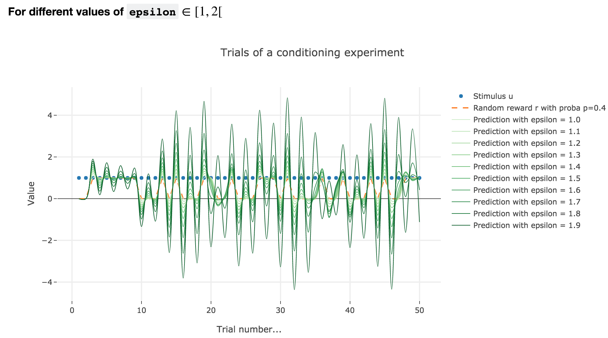
For $ε ∈ [1, 2[$
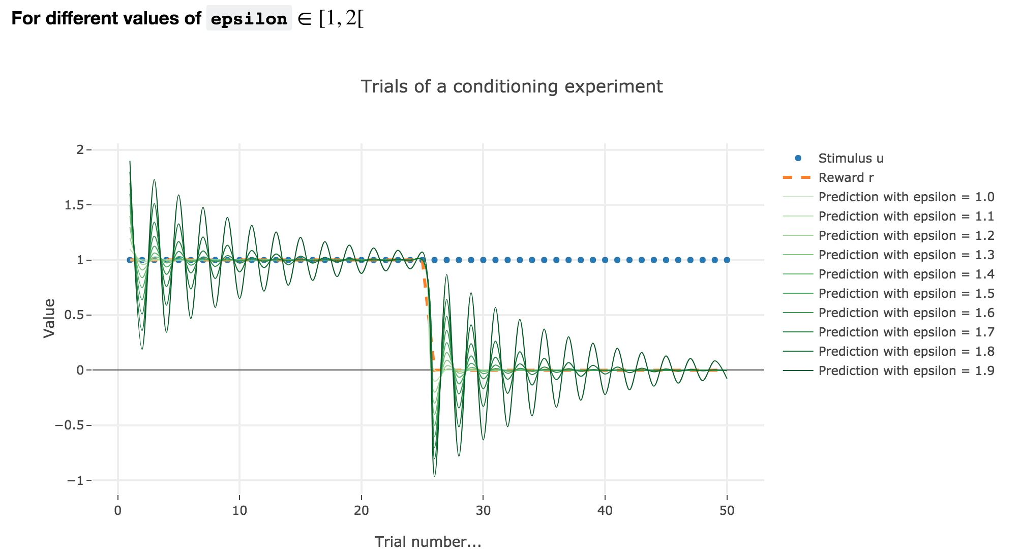
Analogously, if $ε ∈ [1, 2[$: the term $γ ≝ (1-ε) ∈ ]-1, 0]$, and for the first (resp. last) $25$ trials: $w_i = 1 - γ^i$ (resp. $w_i = w_{24} γ^{i-24}$) converges toward the reward $1$ (resp. $0$) while oscillating around it (since $γ ≤ 0$). The oscillation amplitude is all the more significant that $\vert γ \vert$ is big, i.e. that $ε$ is big.
Again, this result can be extended to any constant piecewise reward.
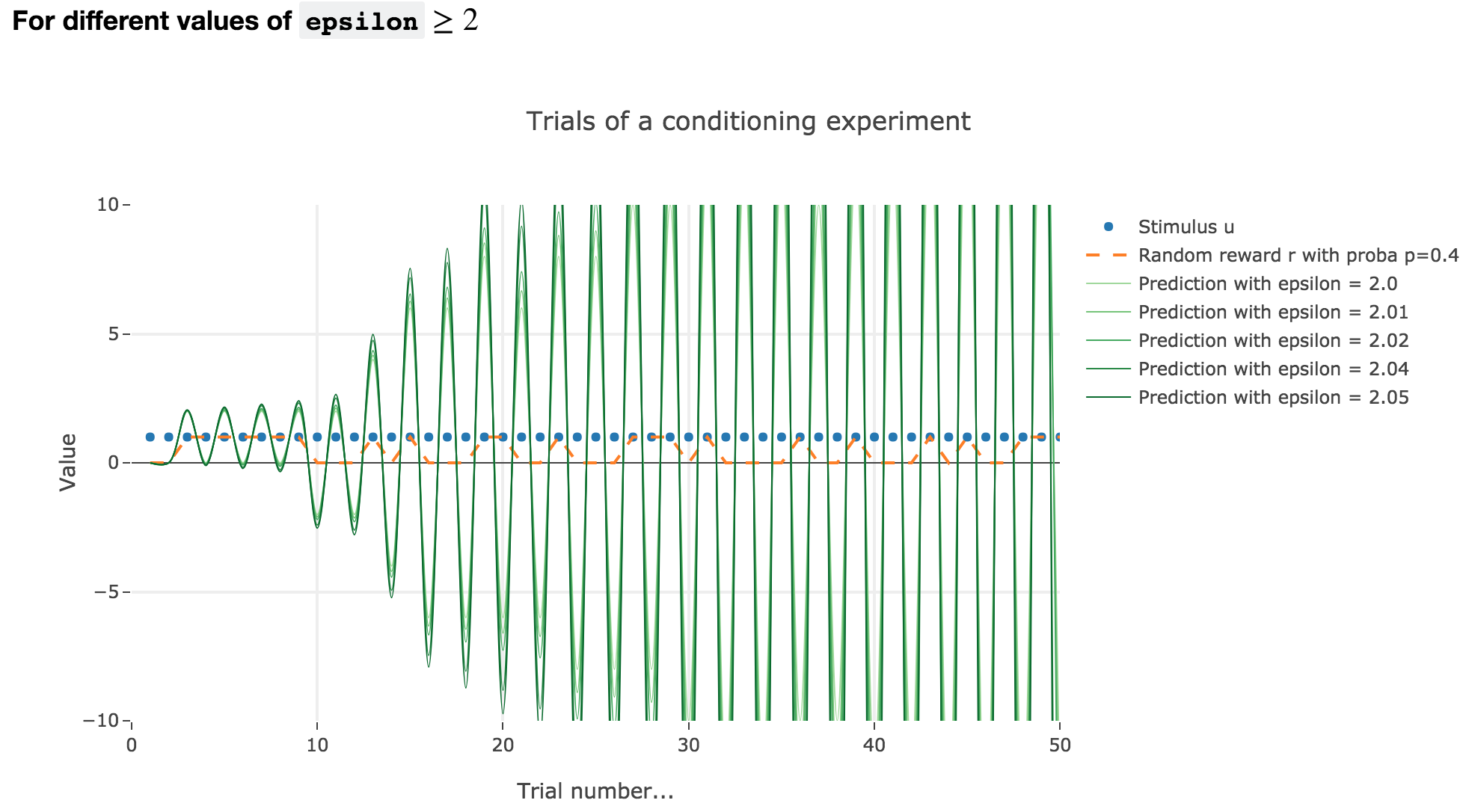
For $ε ≥ 2$
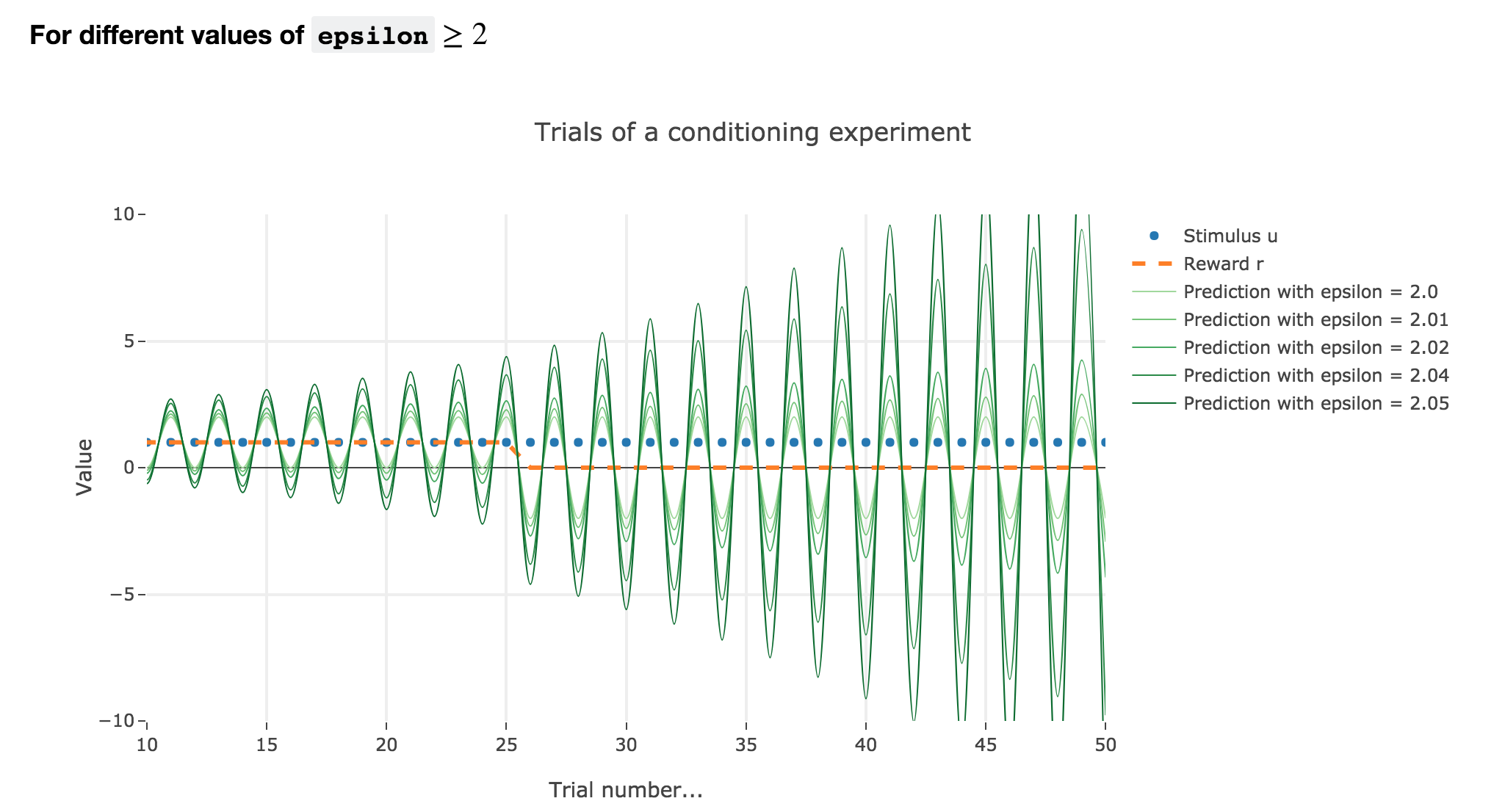
Finally, if $ε ≥ 2$: the term $γ ≝ (1-ε) ≤ -1$, and $w_i$ diverges as $γ^i$ does, while oscillating around it (since $γ ≤ 0$). The oscillation amplitude is all the more significant that $\vert γ \vert$ is big, i.e. that $ε$ is big.
Again, this result stands for any constant piecewise reward.
Going back to our conditioning experiment:
$ε ≤ 1$ corresponds to what is expected from the experiments: the bigger the learning rate, the faster the convergence of the animal prediction, monotonously for a constant reward: hence the name learning rate.
$ε ∈ [1 , 2[$ and $ε ≥ 2$ are both degenerate cases: $ε ≥ 2$ is completely nonsensical from a biological standpoint, and the oscillations of $ε ∈ [1 , 2[$ are not what we want to model, which is rather a convergence of the animal prediction straight to the reward.
2. Partial conditioning
Let us suppose that in each trial, the stimulus is present, but the presence of the reward is a random event with probability $0.4$.
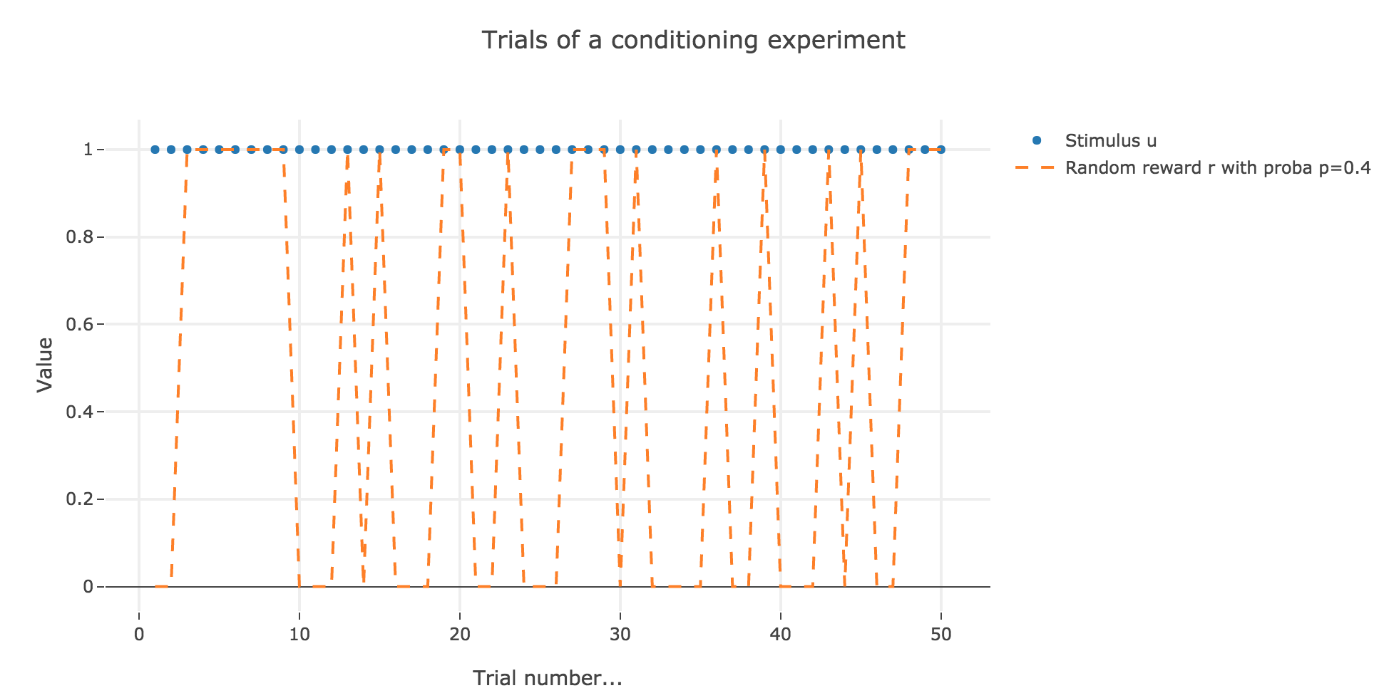
Similarly to what has been done in the previous section:
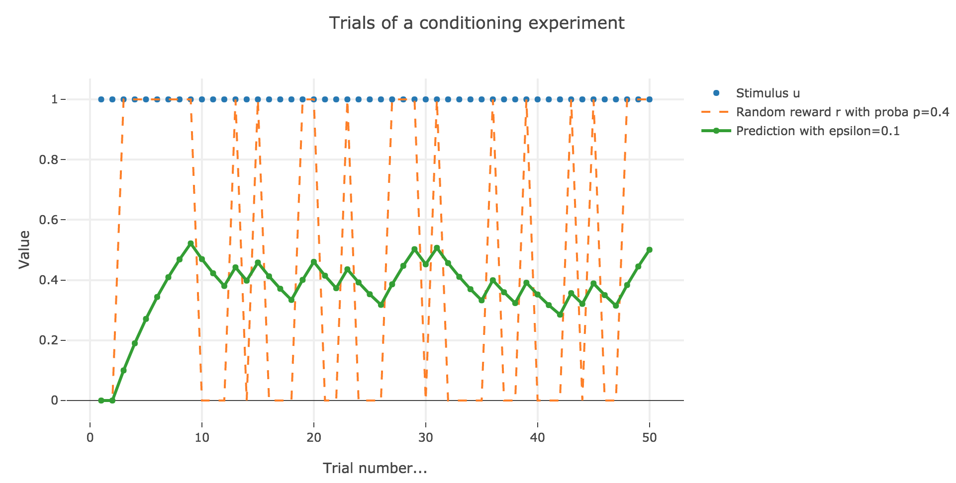
As it happens, the reward is a constant piecewise function, so the previous analysis applies here, by focusing on each segment where the reward is constant (the stimulus is always equal to $1$ here, which simplifies things up). On top of that, we may stress that the shorter these segments are, the higher $ε ≤ 1$ has to be, for the animal to learn the reward within these shorter time spans. The oscillating cases are still irrelevant from a biological standpoint.
3. Blocking
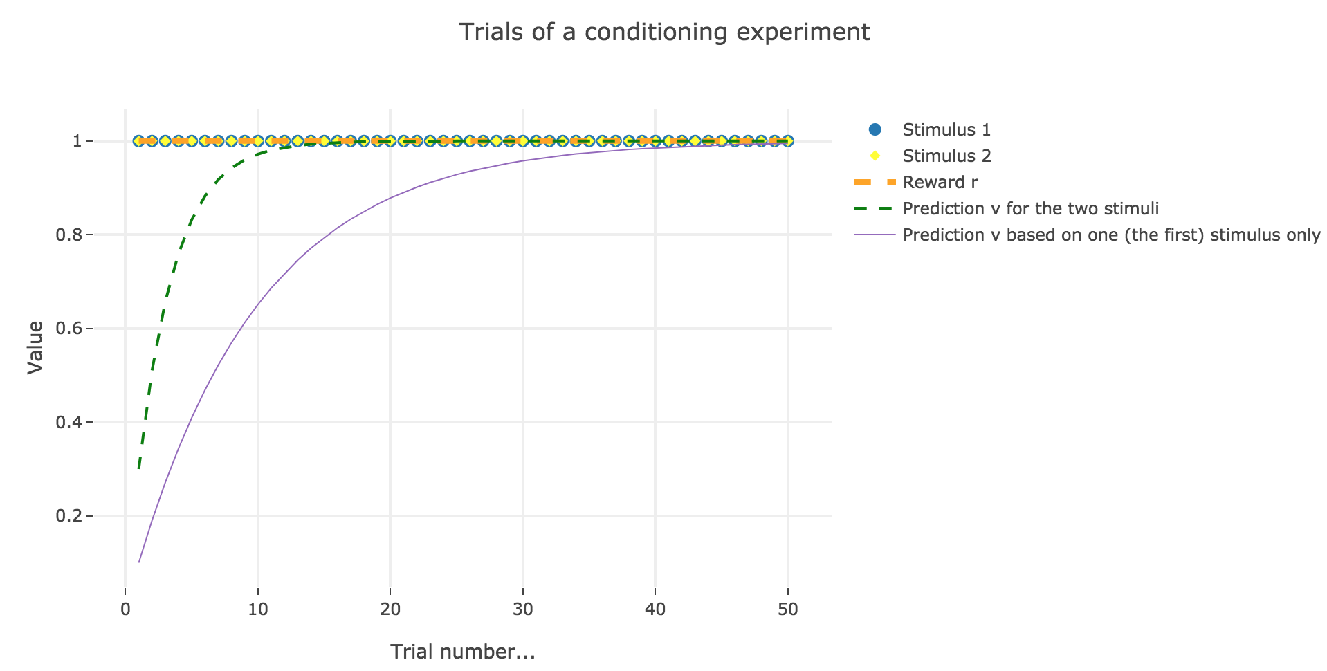
Now, we assume that there are two stimuli, $u_1$ and $u_2$, and two parameters, $w_1$ and $w_2$ to learn, and that the animal prediction is given by $v = w_1 u_1 + w_2 u_2$.
During the first $25$ trials, only one stimulus and the reward are present, during the next $25$ trials, both stimuli and the reward are present.
For the record, here is what happens when there is one single stimulus and $u = r = 1$:
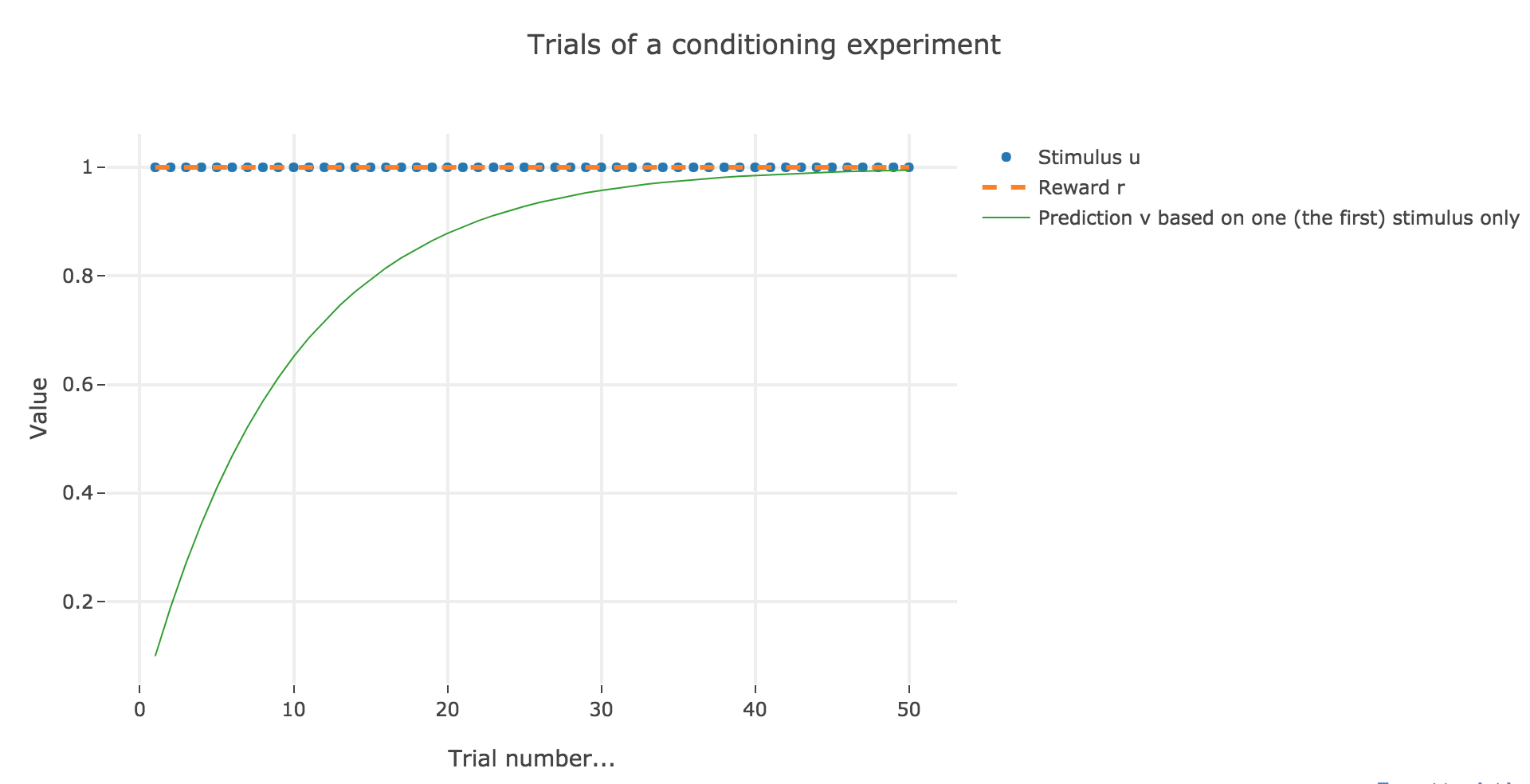
Now, with aforementioned two stimuli:
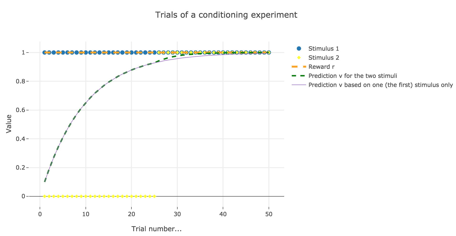
To be more precise, here is the evolution of $w_1$ and $w_2$ throughout the trials:
| Trial | $w_1$ | $w_2$ |
|---|---|---|
| 1 | 0.1 | 0. |
| 2 | 0.19 | 0. |
| 3 | 0.271 | 0. |
| 4 | 0.3439 | 0. |
| 5 | 0.40951 | 0. |
| 6 | 0.468559 | 0. |
| 7 | 0.5217031 | 0. |
| 8 | 0.56953279 | 0. |
| 9 | 0.61257951 | 0. |
| 10 | 0.65132156 | 0. |
| 11 | 0.6861894 | 0. |
| 12 | 0.71757046 | 0. |
| 13 | 0.74581342 | 0. |
| 14 | 0.77123208 | 0. |
| 15 | 0.79410887 | 0. |
| 16 | 0.81469798 | 0. |
| 17 | 0.83322818 | 0. |
| 18 | 0.84990536 | 0. |
| 19 | 0.86491483 | 0. |
| 20 | 0.87842335 | 0. |
| 21 | 0.89058101 | 0. |
| 22 | 0.90152291 | 0. |
| 23 | 0.91137062 | 0. |
| 24 | 0.92023356 | 0. |
| 25 | 0.9282102 | 0. |
| 26 | 0.93538918 | 0.00717898 |
| 27 | 0.94113237 | 0.01292216 |
| 28 | 0.94572691 | 0.01751671 |
| 29 | 0.94940255 | 0.02119235 |
| 30 | 0.95234306 | 0.02413286 |
| 31 | 0.95469547 | 0.02648527 |
| 32 | 0.95657739 | 0.02836719 |
| 33 | 0.95808294 | 0.02987273 |
| 34 | 0.95928737 | 0.03107717 |
| 35 | 0.96025092 | 0.03204071 |
| 36 | 0.96102175 | 0.03281155 |
| 37 | 0.96163842 | 0.03342822 |
| 38 | 0.96213176 | 0.03392156 |
| 39 | 0.96252643 | 0.03431623 |
| 40 | 0.96284216 | 0.03463196 |
| 41 | 0.96309475 | 0.03488455 |
| 42 | 0.96329682 | 0.03508662 |
| 43 | 0.96345848 | 0.03524827 |
| 44 | 0.9635878 | 0.0353776 |
| 45 | 0.96369126 | 0.03548106 |
| 46 | 0.96377403 | 0.03556383 |
| 47 | 0.96384024 | 0.03563004 |
| 48 | 0.96389321 | 0.03568301 |
| 49 | 0.96393559 | 0.03572539 |
| 50 | 0.96396949 | 0.03575929 |
There is a phenomenon of blocking in the sense that: when $u_2$ appears (from the trial $26$ on), the prediction error is already close to zero (the animal has already almost exclusively associated the presence of the reward with the presence of the first stimulus only), so that the second stimulus is hardly taken into account, compared to the first one (hence the blocking).
4. Overshadowing
We still suppose that there are two stimuli and two parameters to learn. However, now:
-
both stimuli and the reward are present throughout all the trials.
-
one of the learning rates is larger: $ε_1 = 0.2$ for the first stimulus, and $ε_2 = 0.1$ for the other one
Here is the evolution of $w_1$ and $w_2$ throughout the trials:
| Trial | $w_1$ | $w_2$ |
|---|---|---|
| 1 | 0.2 | 0.1 |
| 2 | 0.34 | 0.17 |
| 3 | 0.438 | 0.219 |
| 4 | 0.5066 | 0.2533 |
| 5 | 0.55462 | 0.27731 |
| 6 | 0.588234 | 0.294117 |
| 7 | 0.6117638 | 0.3058819 |
| 8 | 0.62823466 | 0.31411733 |
| 9 | 0.63976426 | 0.31988213 |
| 10 | 0.64783498 | 0.32391749 |
| 11 | 0.65348449 | 0.32674224 |
| 12 | 0.65743914 | 0.32871957 |
| 13 | 0.6602074 | 0.3301037 |
| 14 | 0.66214518 | 0.33107259 |
| 15 | 0.66350163 | 0.33175081 |
| 16 | 0.66445114 | 0.33222557 |
| 17 | 0.6651158 | 0.3325579 |
| 18 | 0.66558106 | 0.33279053 |
| 19 | 0.66590674 | 0.33295337 |
| 20 | 0.66613472 | 0.33306736 |
| 21 | 0.6662943 | 0.33314715 |
| 22 | 0.66640601 | 0.33320301 |
| 23 | 0.66648421 | 0.3332421 |
| 24 | 0.66653895 | 0.33326947 |
| 25 | 0.66657726 | 0.33328863 |
| 26 | 0.66660408 | 0.33330204 |
| 27 | 0.66662286 | 0.33331143 |
| 28 | 0.666636 | 0.333318 |
| 29 | 0.6666452 | 0.3333226 |
| 30 | 0.66665164 | 0.33332582 |
| 31 | 0.66665615 | 0.33332807 |
| 32 | 0.6666593 | 0.33332965 |
| 33 | 0.66666151 | 0.33333076 |
| 34 | 0.66666306 | 0.33333153 |
| 35 | 0.66666414 | 0.33333207 |
| 36 | 0.6666649 | 0.33333245 |
| 37 | 0.66666543 | 0.33333271 |
| 38 | 0.6666658 | 0.3333329 |
| 39 | 0.66666606 | 0.33333303 |
| 40 | 0.66666624 | 0.33333312 |
| 41 | 0.66666637 | 0.33333318 |
| 42 | 0.66666646 | 0.33333323 |
| 43 | 0.66666652 | 0.33333326 |
| 44 | 0.66666656 | 0.33333328 |
| 45 | 0.6666666 | 0.3333333 |
| 46 | 0.66666662 | 0.33333331 |
| 47 | 0.66666663 | 0.33333332 |
| 48 | 0.66666664 | 0.33333332 |
| 49 | 0.66666665 | 0.33333332 |
| 50 | 0.66666665 | 0.33333333 |
There is a phenomemon of overshadowing: the first stimulus ends up being taken into account twice as much as the second (overshadowing it), as it has been learned at a rate two times bigger.
Leave a comment