Tutorial 3: Regression
Tutorial 3: Regression
Kexin Ren & Younesse Kaddar (Lecturer: Nicolas Perrin)
\[\newcommand{\T}{ {\raise{0.7ex}{\intercal}}}\]In this lab, we aim to create a model out of experimental data. The model structure is established in advance, and the parameter thereof are gradually modified. In Machine Learning (ML), it is a crucial technique, as modifying the parameters on the fly leads to performance improvement over time.
Most of the time, the goal is to model correlations, which will enable us to make predictions by completing partial data.
Typically, one attempts at performing regressions on stongly-correlated data, but there exist numerous ways to do it, with different levels of complexity, and sometimes the crux of the issue is to model the uncertainty and the data variance. The most simple case is the one of linear regression (that should be called “affine regression”), in which a relation of this form is assumed:
\[\textbf{y} = A \textbf{x} + \textbf{b}\]between data $\textbf{x}$ and $\textbf{y}$ (in a more formal probabilistic setting: the relation pertains to the conditional expectancy of $\textbf{y}$ given $\textbf{x}$).
Many methods can be used to adjust the parameters $A$ and $\textbf{b}$, the most well-known of which being the least squares one.
Oftentimes, linear models are not enough. In this lab, we will go over a few methods going further (while remaining in a non-probabilistic setting). The aim is to observe a set of data
\[\big\lbrace (\textbf{x}^{(i)}, \textbf{y}^{(i)}) \big\rbrace\]and design a model
\[\textbf{y} = f(\textbf{x})\]written as a sum of $k$ functions depending on parameters $θ_i$:
\[f(\textbf{x}) = \sum\limits_{ i=1 }^k f_{θ_i}(\textbf{x})\]In what follows, $\textbf{y}$ will be assumed to be of dimension $1$ (and hence will be written $y$).
1. Weighted sum of Gaussian functions
In this part, the $f_{θ_i}$ functions will be of the form:
\[f_{θ_i} ≝ θ_i \; \underbrace{\exp\left(- \frac{(\textbf{x}-\textbf{c}_i)^2}{σ_i^2}\right)}_{≝ \; ϕ_i(\textbf{x})}\]And one sets:
\[ϕ(\textbf{x}) ≝ \Big(ϕ_1(\textbf{x}) \; ⋯ \; ϕ_k(\textbf{x})\Big)^\T\\ θ ≝ \big(θ_1 \; ⋯ \; θ_k\big)^\T\]so that:
\[f(\textbf{x}) = ϕ(\textbf{x})^\T θ\]The goal of this regression is to adjust $θ$. We will see 3 methods: two incremental algorithms, and a batch one, that treats all the data in one go.
1.1. Gradient descent (incremental method)
Let us denote by $θ^{(t)}$ the value of the parameters at step $t$. One observes a new data point:
\[\big(\textbf{x}^{(t+1)},\; y^{(t+1)}\big)\]The estimation error on this data point is the following:
\[ε^{(t+1)} = y^{(t+1)} - f_{θ^{(t)}}\left(x^{(t+1)}\right)\]The bottom line of gradient descent is to sightly modify $θ$ to improve the resulting error on the last data point. For this purpose, consider the function
\[θ ⟼ y^{(t+1)} - f_θ(\textbf{x}^{(t+1)})\]and compute its gradient at $θ^{(t)}$:
\[\nabla_θ^{(t+1)} = - ε^{(t+1)}ϕ(\textbf{x}^{(t+1)})\]The gradient is oriented toward the maximal slope, giving the direction leading to the steepest increase of the function. So if $ε^{(t+1)}$ is to be decreased, it’s in the opposite direction of the gradient that $θ$ should be modified:
\[θ^{(t+1)} = θ^{(t)} + α ε^{(t+1)}ϕ(\textbf{x}^{(t+1)})\]where $α > 0$ is a learning rate.
Instructions:
Open the exoGD.py file. It contains the function generateDataSample(x) which makes it possible to generate a noise data $y$ for $\textbf{x} ∈ [0, 1]$ ($\dim(x) = 1$), the function phiOutput(input) which allows us to generate the vector $ϕ(\textbf{x})$ or a matrix of vectors $ϕ(\textbf{x}^{(i)})$ concatenated if the input is a tuple, and the function f(input, *user_theta) which makes it possible to compute $f(\textbf{x})$. The parameters used by f are either the global variable theta, or an input value *user_theta. The number of coordinates of $ϕ(\textbf{x})$ (that is, the number $k$ of Gaussian functions) is defined by the global variable numFeatures.
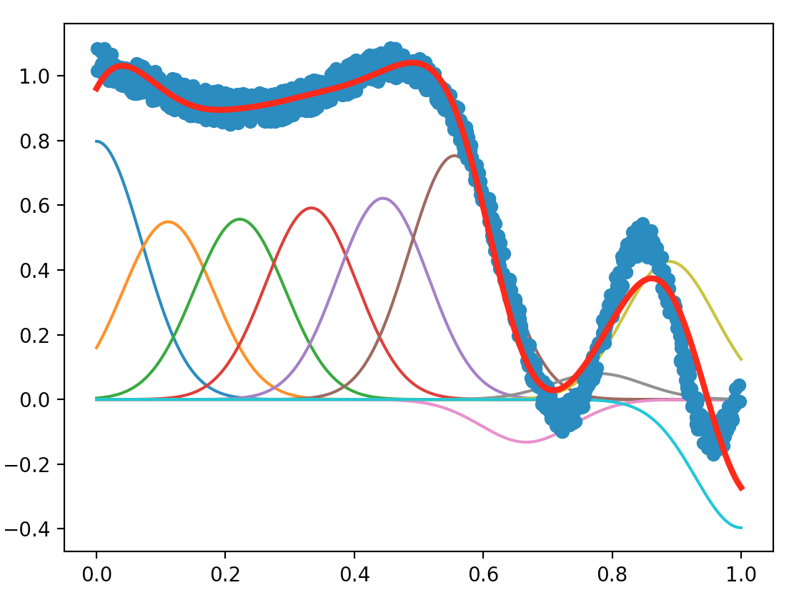
Implement the train_GD(maxIter) function that will adjust the theta value by gradient descent from a data number equal to maxIter. When the file is executed, the observed data is displayed by dots, and the red curve is the “learned” function, that is, the function f corresponding to the parameters theta adjusted by train_GD(maxIter). Other curves correspond to the different $f_{θ_i}(\textbf{x})$ and show how the function f is decomposed.
According to the formulas given in the tutorial to compute $f$, $ε$, the gradient and theta, we modify the original code as follows for the train_GD(maxIter) function:
    alpha = 0.9

    # [...]

	def train_GD(maxIter):
	global theta, xHistory, yHistory, alpha
	iterationCount = 0

		# Draw a random sample on the interval [0,1]

	while iterationCount < maxIter:
		#----------------------#
		#  Training Algorithm  #
		#----------------------#
		x = np.random.random()
		y = generateDataSample(x)
		xHistory.append(x)
		yHistory.append(y)

		#-----------------------------#
		#         Modification        #
		#-----------------------------#
		fval = f(x)
		e = y - fval
		delta = phiOutput(x)
		theta += alpha*e*delta


		#-----------------------------#
		#  End of Training Algorithm  #
		#-----------------------------#
		iterationCount += 1
With maxIter = $1000$, numFeatures = $10$ and alpha = $0.9$, the plot we obtained is shown as below.

Try to find values of maxIter, numFeatures and of learning rate leading that lead to good results (you can put screenshots in your report).
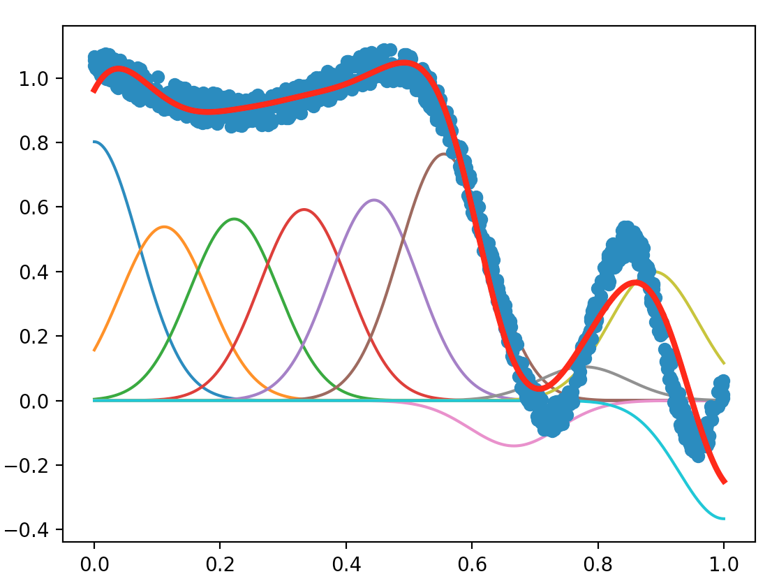
We first tested the effect of maxIter by setting maxIter = $100$, $1000$ (original), and $10000$, keeping numFeatures = $10$ and alpha = $0.9$. The plots are shown as follows:
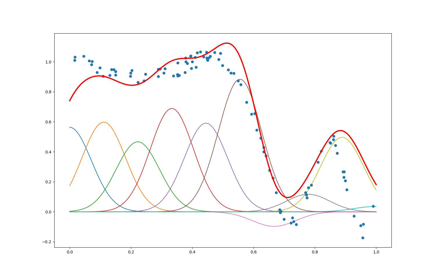

The number of data points maxIter is also the number of times we update the $θ$ estimator along the opposite of the gradient of the error $y - f_θ(\textbf{x})$. We can see that:
-
When
maxIter$=100$: there hasn’t been enough data points/updates of $θ$ for the predictor $f(\textbf) ≝ ϕ(\textbf{x})^\T θ$ to match the shape of the $y$ output (especially when $\textbf{x}$ ranges from $0$ to $0.5$): too few data points leads to underfitting -
When
maxIter$=10000$: the predictor $f(\textbf)$ doesn’t match the output as well as whenmaxIter$=1000$, especially when $\textbf{x}$ ranges from $0.6$ to $1$: too many data points leads to overfitting
The best compromise is met for an intermediary number of data points (as it happens: when maxIter $=1000$ here).
Then, we tested the effect of numFeatures by setting numFeatures = $5$, $10$ (original), $15$ and $30$, keeping maxIter = $1000$ and alpha = $0.9$. The plots are shown as follows:
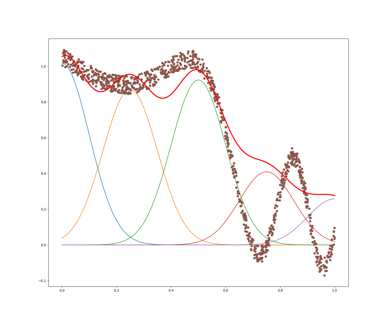


We can see that, as the number of features increases, the redline fits the sample points better at first. But with too many number of features, the redline overfits the sample points. Indeed: even though the predictor matches the data better for numFeatures $= 15$ than numFeatures $= 10$ when $\textbf{x} ≥ 0.7$ (the bell-shaped curve is perfectly fitted), the overfitting is already conspicuous at $15$ features for $\textbf{x} ≤ 0.5$: the predictor tends to overcomplicate the shape of the output, that is seen to be smoothly approximable. Thus, using an appropriate number of features is very important.
Finally, we tested the effect of alpha by setting alpha = $0.1$, $0.5$, and $0.9$, keeping maxIter = $1000$ and numFeatures = $10$. The plots are shown as follows:


Let us recall that $α$ is the learning rate: that is, $α$ specifies how much one goes along the opposite direction of the gradient (toward a local minimum) at each step. We can see that:
-
for a value of $α$ too low: the steps along the opposite of the gradient have been so small that the prediction error $y - ϕ(\textbf{x})^\T θ$ at the end of the iterations hasn’t been locally minimized yet
-
for a value of $α$ too high: the steps along the opposite of the gradient are so big than the local minimum might have been missed by a step going “too far”
Again, we have to strike a balance between a low learning rate (more likely to hit a local minimum, but slower algorithm) and a high one (faster algorithm, but more likely to miss the targeted local minimum by making steps along the gradient that are too big).
1.2 Least squares (batch method)
This time, we consider a data set of size $N$:
\[\big\lbrace (\textbf{x}^{(i)}, \textbf{y}^{(i)}) \big\rbrace_{1 ≤ i ≤ N}\]and we try to minimize the following error:
\[ε(θ) ≝ \frac 1 {2N} \sum\limits_{ i=1 }^N \left(y^{(i)} - f_θ\big(\textbf{x}^{(i)}\big)\right)^2\]A local minimum $θ$ corresponds to a zero gradient:
\[\textbf{0} = \nabla ε(θ) = - \frac 1 N \sum\limits_{ i=1 }^N ϕ(\textbf{x}^{(i)}) \left(y^{(i)} - ϕ(\textbf{x}^{(i)})^\T θ\right)\]i.e.
\[\underbrace{\left(\sum\limits_{ i=1 }^N ϕ(\textbf{x}^{(i)}) ϕ(\textbf{x}^{(i)})^\T \right)}_{≝ \; A} \; θ = \underbrace{\sum\limits_{ i=1 }^N ϕ(\textbf{x}^{(i)}) y^{(i)}}_{≝ \; b}\]Therefore:
\[θ = A^\sharp b\]where $A^\sharp$ is the pseudo-inverse of $A$.
Instructions:
Open the exoLS.py file. Its structure is similar to exoGD.py, but the data points are generated in one go instead of being built up incrementally. The lines where you can see that are the following one: x = np.random.random(1000) (the number of data points can be changed) and y = map(generateDataSample, x).
Implement the function train_LS() which computes theta according to the least squares method.
In compliance with the batch method, with the given fomulas of A, b and theta, we modify the function train_LS(maxIter) as follows:
def train_LS():
	global x, y, numfeatures, theta
	#----------------------#
	# # Training Algorithm ##
	#----------------------#

	A = np.zeros(shape=(numFeatures, numFeatures))
	b = np.zeros(numFeatures)

	# LES MODIFICATIONS SONT A FAIRE ICI ---------------------------------------------------------

	for i in range(1000):
        A += np.outer(phiOutput(x[i]),phiOutput(x[i]))
        b += phiOutput(x[i])*y[i]

	theta = np.dot(np.linalg.pinv(A),b)

	#-----------------------------#
	# # End of Training Algorithm ##
	#-----------------------------#
A faster way to do it is as follows:
def train_LS():
	global x, y, numfeatures, theta
	#----------------------#
	# # Training Algorithm ##
	#----------------------#

	Phi = phiOutput(x)
	A = Phi.dot(Phi.T)
	b = Phi.dot(y)

	theta = np.dot(np.linalg.pinv(A),b)
Indeed,
\[\begin{align*} A &= \sum\limits_{ i=1 }^N ϕ(\textbf{x}^{(i)}) ϕ(\textbf{x}^{(i)})^\T \\ &= \underbrace{\begin{pmatrix} ϕ(\textbf{x}^{(1)}) \mid ⋯ \mid ϕ(\textbf{x}^{(N)}) \end{pmatrix}}_{= \; \texttt{phiOutput(x)}} \begin{pmatrix} ϕ(\textbf{x}^{(1)}) \mid ⋯ \mid ϕ(\textbf{x}^{(N)}) \end{pmatrix}^\T \\ &= \texttt{phiOutput(x)} \; \texttt{phiOutput(x)}^\T \end{align*}\]and
\[\begin{align*} b &= \sum\limits_{ i=1 }^N ϕ(\textbf{x}^{(i)}) y^{(i)} \\ &= \begin{pmatrix} ϕ(\textbf{x}^{(1)}) \mid ⋯ \mid ϕ(\textbf{x}^{(N)}) \end{pmatrix} \begin{pmatrix} y^{(1)} ⋯ y^{(N)} \end{pmatrix}^\T\\ &= \texttt{phiOutput(x)} \; y \end{align*}\]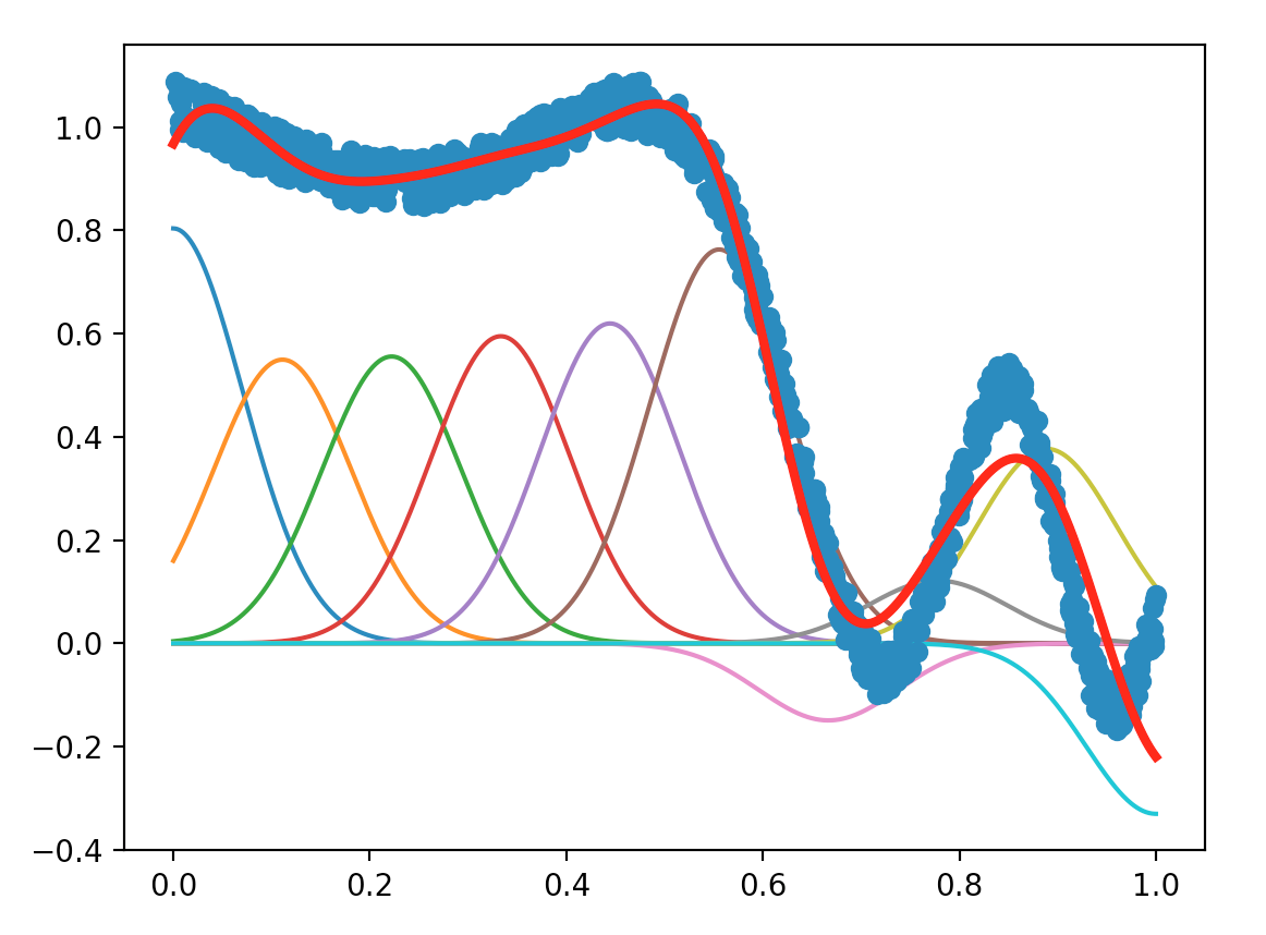
Try to find new parameters that lead to good results.
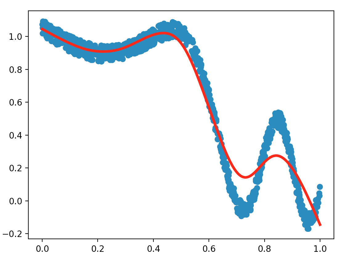
The plots of LS method with different values for the parameters numFeatures and maxIter are shown as below:


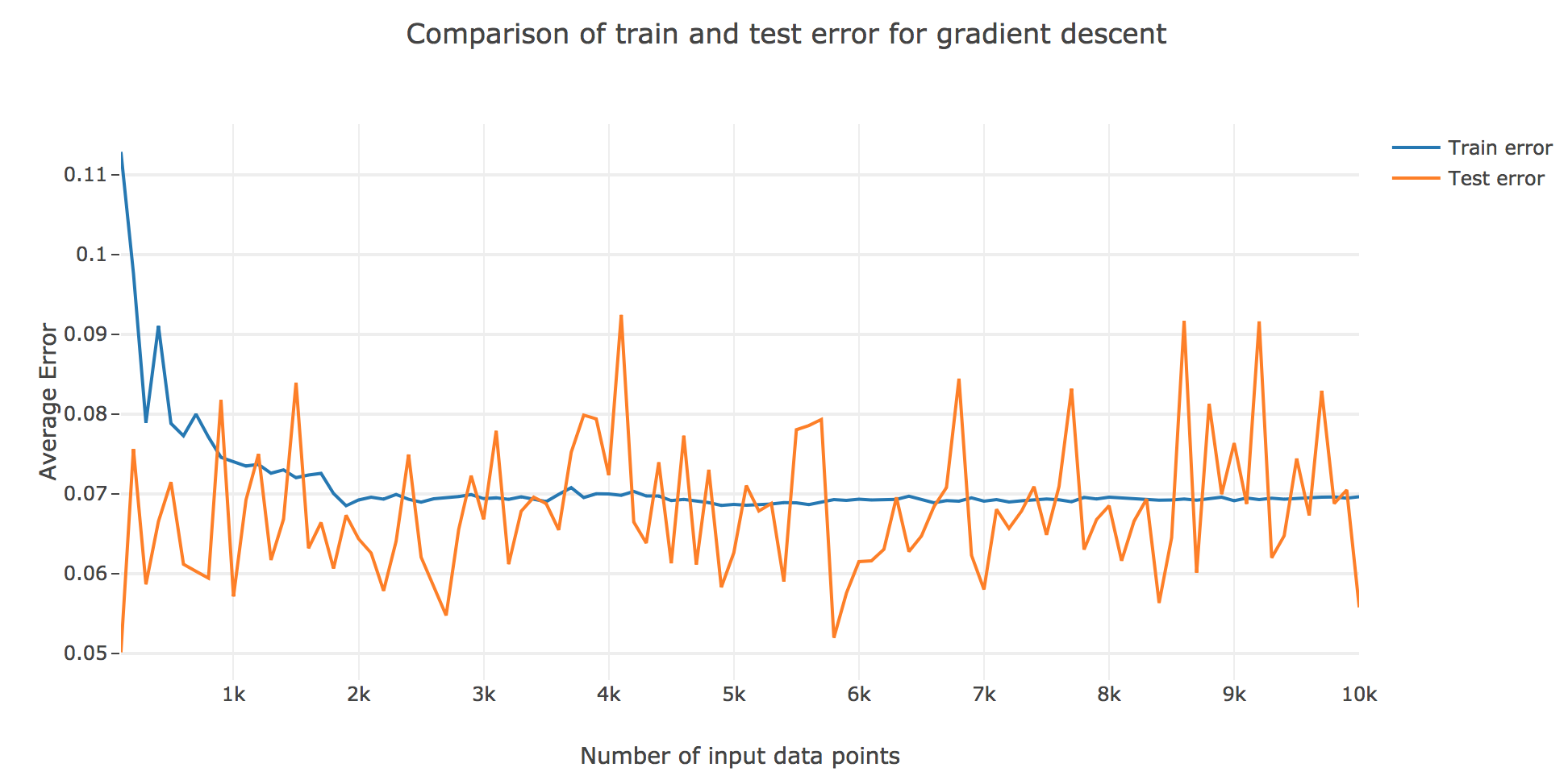
We summarized the average error regarding the values of numFeatures and maxIter in the following figures:

The figures all above illustrate that higher number of features contribute to lower average error, and when the number of features exceed 15, the improvement of the accuracy is not significant anymore. Thus, for the sake of saving time, we may infer that a good value for numFeatures could be 15.

From the figure we can see that, the average error goes down when number of data points exceed 1000. Thus, with about 1000 data points, we can get a relatively low average error, as well as a ideal execution speed. Though the lowest error appears around 300 points, such a small scale data is not a reasonable choice to get a good model.
Now that you’ve been able to test an incremental method and a batch method, what do you think are the advantages and drawbacks of the least-squares approach?
We first tested the execution time of the two methods (see chart below, alpha = 0.1), and we found that, with the same parameters, the batch method (with given codes) is slower than the incremental method.
| Method | numFeatures = $5$, maxIter = $1000$ |
numFeatures = $10$, maxIter = $1000$ |
numFeatures = $10$, maxIter = $10000$ |
|---|---|---|---|
| incremental | $0.031$ sec | $0.031$ sec | $0.297$ sec |
| batch | $0.047$ sec | $0.032$ sec | $0.391$ sec |
We also tested the accuracy of the two methods by calculating average error (i.e. the sum of the absolute values of errors devided by number of data points), as shown in the following chart (alpha = 0.1). We found that, with the same parameters, the batch method is more accurate than the incremental method.
| Method | numFeatures = $5$, maxIter = $1000$ |
numFeatures = $10$, maxIter = $1000$ |
numFeatures = $10$, maxIter = $10000$ |
|---|---|---|---|
| incremental | $0.115$ | $0.072$ | $0.055$ |
| batch | $0.095$ | $0.053$ | $0.051$ |
Moreover, when the number of data points is very high, the difference between the average error of the two methods became small, inferring that the incremental method may require lots of data points for a good accuracy.
Besides, when solving for the linear system in one go (our second version codes), with small number of points (about below $1000$), GD method is faster; however, with high number of points, LS is the faster one. Thus, it becomes more advantageous for a larger number of data points, as it relies on the fact that numpy is faster than regular python, as it is implemented in C under the hood.

1.3 Recursive Least Squares Algorithm (incremental method)
The recursive least squares algorithm is another incremental method in which $A$ and $b$ are computed at each iteration on a new data point (as $A$ and $b$ can be regarded as sums over the data points):
\[A^{(t+1)} = A^{(t)} + ϕ(\textbf{x}^{(t+1)})ϕ(\textbf{x}^{(t+1)})^T\\ b^{(t+1)} = b^{(t)} + ϕ(\textbf{x}^{(t+1)}) y^{(t+1)}\]The parameters
-
can be directly obtained with:
\[θ^{(t+1)} = \big(A^{(t+1)}\big)^\sharp \; b^{(t+1)}\] -
can be estimated with resort to the Sherman-Morrison lemma (provided $A^{(0)}$ is non-zero):
\[\left(A + uv^T\right)^\sharp = A^\sharp - \frac{A^\sharp uv^T A^\sharp}{1+v^T A^\sharp u}\]
Instruction:
Open the exoRLS.py file. Its structure is very similar to exoGD.py.
Implement the train_RLS() function which will incrementally adjust theta by following the least-squares recursive method (without using Sherman-Morrison’s lemma), and show in your report the obtained results.
Without Sherman-Morrison’s lemma: According to the formulas given in the instruction to compute A, b and theta, we modify the function train_RLS(maxIter) as below:
def train_RLS(maxIter):
	global theta, xHistory, yHistory

	## Initialize A and b ##
	A = np.zeros(shape=(numFeatures,numFeatures))
	b = np.zeros( numFeatures )

	iterationCount = 0
	# Begin training
	while iterationCount < maxIter:

		# Draw a random sample on the interval [0,1]
		x = np.random.random()
		y = generateDataSample(x)
		xHistory.append(x)
		yHistory.append(y)

		#----------------------#
		## Training Algorithm ##
		#----------------------#

		phi = phiOutput(x)
		A += np.outer(phi, phi)
		b += phi.dot(y)

		#-----------------------------#
		## End of Training Algorithm ##
		#-----------------------------#

		iterationCount+=1

	theta = np.dot(np.linalg.pinv(A),b)
The plot we obtain is shown below:
Open the exoRLS2.py file, and this time implement the least recursive square method using the Sherman-Morrison lemma.
First, we define pseudo-inversed $A^{\sharp}$ as
A_sharp = np.eye(numFeatures)
Then, with the formulas given before and the Sherman-Morrison lemma, we modify the train_RLS(maxIter) function as below:
def train_RLS(maxIter):
	global theta, xHistory, yHistory

	## Initialize b and A_sharp ##
	b = np.zeros( numFeatures )
	A_sharp = np.eye(numFeatures)

	iterationCount = 0
	# Begin training
	while iterationCount < maxIter:

		# Draw a random sample on the interval [0,1]
		x = np.random.random()
		y = generateDataSample(x)
		xHistory.append(x)
		yHistory.append(y)

		#----------------------#
		## Training Algorithm ##
		#----------------------#

		phi = phiOutput(x)

		A_sharp -= A_sharp.dot(np.outer(phi, phi).dot(A_sharp))/(1+phi.dot(A_sharp.dot(phi)))
		b += phi.dot(y)

		#-----------------------------#
		## End of Training Algorithm ##
		#-----------------------------#

		iterationCount+=1

	theta = np.dot(A_sharp,b)
With the Sherman-Morrison lemma, the plot we obtain is shown below:
Compare the two variants (with or without the Sherman-Morrison lemma). Which is the most accurate, which is the fastest, and why (can you include in your report measurement of computing time)?
We first compared the time of execution with different maxIter of the two methods (with or without the Sherman-Morrison lemma). The results are shown in the following chart:
| Method | numFeatures = $5$, maxIter = $1000$ |
numFeatures = $10$, maxIter = $1000$ |
numFeatures = $10$, maxIter = $10000$ |
|---|---|---|---|
| w/o Sherman-Morrison lemma | $0.13$ sec | $0.14$ sec | $1.38$ sec |
| with Sherman-Morrison lemma | $0.06$ sec | $0.06$ sec | $0.64$ sec |
It demonstrated that the method with Sherman-Morrison lemma is faster than the one without Sherman-Morrison lemma.
Then we compared the accuracy of the two methods by calculating the average squared errors. the results are shown as below (the values in the chart are magnified $10^5$ times):
| Method | numFeatures = $5$, maxIter = $1000$ |
numFeatures = $10$, maxIter = $1000$ |
numFeatures = $10$, maxIter = $10000$ |
|---|---|---|---|
| w/o Sherman-Morrison lemma | $2$ | $1$ | $0.1$ |
| with Sherman-Morrison lemma | $5$ | $0.6$ | $0.02$ |
It demonstrated that with higher numFeatures and higher maxIter, the accuracy of the method with Sherman-Morrison lemma increases. When numFeatures is too low, the accuracy of the method with Sherman-Morrison lemma may be lower than the other. However, with higher numFeatures, the accuracy of the method with Sherman-Morrison lemma could lead to higher accuracy.


2 LWLS: Locally-Weighted Least-Squares (batch method)
The LWLS algorithm resorts to a weighted sum of local linear models, parametrized by $θ_i$ vectors such that $\dim θ_i = \dim \textbf{x} + 1 = d + 1$:
\[f(\textbf{x}) = \sum\limits_{ i=1 }^k \tfrac{ϕ_i(\textbf{x})}{\sum\limits_{ j=1 }^k ϕ_j(\textbf{x})} \; m_{θ_i}(\textbf{x})\]where
- $m_{θ_i}(\textbf{x}) = w(\textbf{x})^\T θ_i$
- $w(\textbf{x}) = (\textbf{x}_1 \; ⋯ \; \textbf{x}_d \, 1)^\T$
Each local model is computed thanks to the following local weighted error:
\[ε_i(θ_i) = \frac 1 {2N} \sum\limits_{ j=1 }^N ϕ_i(\textbf{x}^{(j)}) \Big(y^{(j)} - \underbrace{m_{θ_i}(\textbf{x}^{(j)})}_{= w(\textbf{x})^\T θ_i}\Big)^2\]As for the least squares method, we set the corresponding gradient to zero, which leads to:
\[\begin{align*} & \textbf{0} = - \frac 1 N \sum\limits_{ j=1 }^N ϕ_i(\textbf{x}^{(j)}) w(\textbf{x}^{(j)}) \big(y^{(j)} - w(\textbf{x}^{(j)})^\T θ_i\big) \\ ⟺ \quad & \underbrace{\sum\limits_{ j=1 }^N ϕ_i(\textbf{x}^{(j)}) \, w(\textbf{x}^{(j)}) \, w(\textbf{x}^{(j)})^\T}_{≝ \; A_i} \; θ_i = \underbrace{\sum\limits_{ j=1 }^N ϕ_i(\textbf{x}^{(j)}) w(\textbf{x}^{(j)}) y^{(j)}}_{≝ \; b_i} \\ ⟹ \quad & θ_i = A_i^\sharp \, b_i \end{align*}\]Instructions
Open the file exoLWLS.py. It contains the functions generateDataSample(x), phiOutput(input), and the f(input) function, which is different this time: it resorts to w(input) to compute the $w(\textbf{x})$ for one or several $\textbf{x}$ value(s). Note that, from now on, theta is a matrix formed by the horizontal concatenation of the $θ_i$, which are themselves $2$-dimensional vectors (since we assume that $\dim \textbf{x} = 1$).
Implement the function train_LWLS() which computes theta. Again, show the results in your report.
Similarly to what we did for the Least Squares method:
\[\begin{align*} A_i &= \sum\limits_{ j=1 }^N ϕ_i(\textbf{x}^{(j)}) \, w(\textbf{x}^{(j)}) \, w(\textbf{x}^{(j)})^\T \\ &= \underbrace{\begin{pmatrix} \textbf{x}_1^{(1)} & ⋯ & \textbf{x}_1^{(N)} \\ 1 & ⋯ & 1 \\ \end{pmatrix}}_{≝ \; W(\textbf{x})} \underbrace{\begin{pmatrix} ϕ_i(\textbf{x}^{(1)}) & \\ & \ddots \\ & & ϕ_i(\textbf{x}^{(N)}) \end{pmatrix}}_{≝ \; \texttt{diag}\big(ϕ_i(\textbf{x}^{(j)})\big)_{1 ≤ j ≤ N}} \begin{pmatrix} \textbf{x}_1^{(1)} & ⋯ & \textbf{x}_1^{(N)} \\ 1 & ⋯ & 1 \\ \end{pmatrix}^\T \\ &= W(\textbf{x}) \; \texttt{diag}\big(ϕ_i(\textbf{x}^{(j)})\big)_{j} \; W(\textbf{x})^\T \end{align*}\]and likewise:
\[b_i = W(\textbf{x}) \; \texttt{diag}\big(ϕ_i(\textbf{x}^{(j)})\big)_{j} \; \textbf{y}\]which yields:
def train_LWLS():
	global x, y, numfeatures, theta

	#----------------------#
	## Training Algorithm ##
	#----------------------#

	Phi = phiOutput(x)
	W = w(x)

	for k in range(numFeatures):
		Wphi = W.dot(np.diag(Phi[k]))
		A_i = Wphi.dot(W.T)
		b_i = Wphi.dot(y)
		theta[:,k] = np.dot(np.linalg.pinv(A_i),b_i)

	#-----------------------------#
	## End of Training Algorithm ##
	#-----------------------------#

train_LWLS()
For similar parameters, compare the results obtained with the LWLS method and the least squares one (exoLS.py). Which method is the fastest, and which one gives the best results according to you? What are the main differences if we were to increase numfeatures for example?
With the LS method, one tries to approximate the output vector $\textbf{y} ≝ (y^{(1)} ⋯ y^{(N)})^\T$ by the predictor:
\[f(\textbf{x}) = \underbrace{Φ^\T}_{\rlap{\text{design matrix}}} \overbrace{θ}^{\text{estimator}}\]where
\[\begin{cases} Φ ≝ \big(ϕ_i(\textbf{x}^{(j)})\big)_{\substack{1 ≤ i ≤ k \\ 1 ≤ j ≤ N}} ∈ 𝔐_{k, N}(ℝ) \\ θ ∈ 𝔐_{k, 1}(ℝ) \end{cases}\]As it happens, the “best” estimator $θ$, i.e. the one that minimizes the squared error (the squared euclidean distance between the predictor and the output):
\[\Vert \textbf{y} - Φ^\T θ\Vert_2^2\]is given by (as shown before):
\[θ ≝ (Φ Φ^\T)^\sharp Φ \textbf{y}\]In the LWLS case: for each estimator $θ_i$, each data point $\textbf{x}^{(j)}$ is given the weight $ϕ_i(\textbf{x}^{(j)})$ (recall that $\dim \textbf{x}^{(j)} = 1$ for all $1 ≤ j ≤ N$), where $ϕ_i$ is a Gaussian of mean $\textbf{c}_i$ and of standard deviation $σ_i$. Consequently, $θ_i$ is the “best” estimator (i.e. minimizing the corresponding weighted squared error) given those weights.
The resulting predictor is set to be:
\[f(\textbf{x}) = \sum\limits_{ i=1 }^k \overbrace{λ_i}^{≝ \; ϕ_i(\textbf{x})\big/\sum\limits_{ j=1 }^k ϕ_j(\textbf{x})} \; \big(\textbf{x}_1 \; ⋯ \; \textbf{x}_d \; 1\big) θ_i\]that is: the higher the weight the estimator $θ_i$ gives to $\textbf{x}$, the higher the coefficient $λ_i$ is in the weighted sum defining $f(\textbf{x})$, and hence the more $θ_i$ is taken into account to predict the ouput at $\textbf{x}$
As for the execution speed for both of these models: as shown in the figure below, by averaging over many trials we found that, as the number of data points increases, the execution time of LWLS become more and more longer than that of LS. Thus, normally, LS is the faster one.

As for the accuracy (the higher the accuracy, the lower test/train error): as shown in the figures below comparing the train/test errors on all the models, LWLS doesn’t seem to perform as good as LS (as its errors are higher):

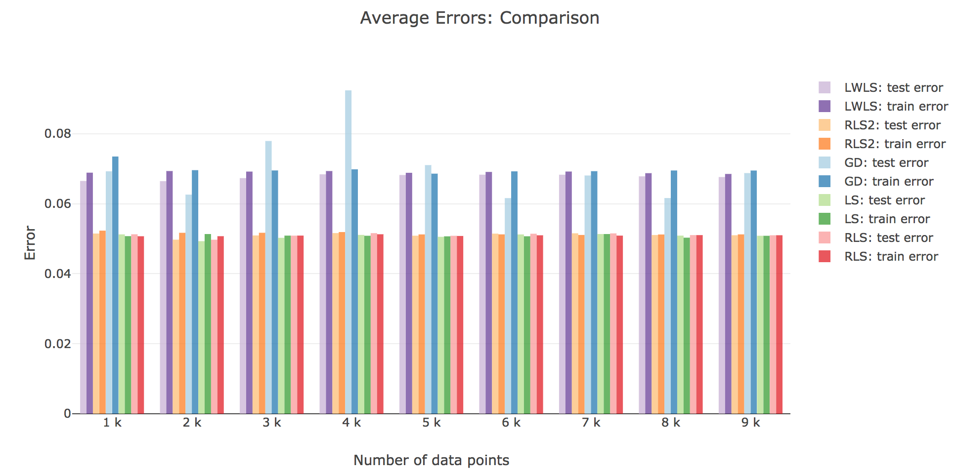
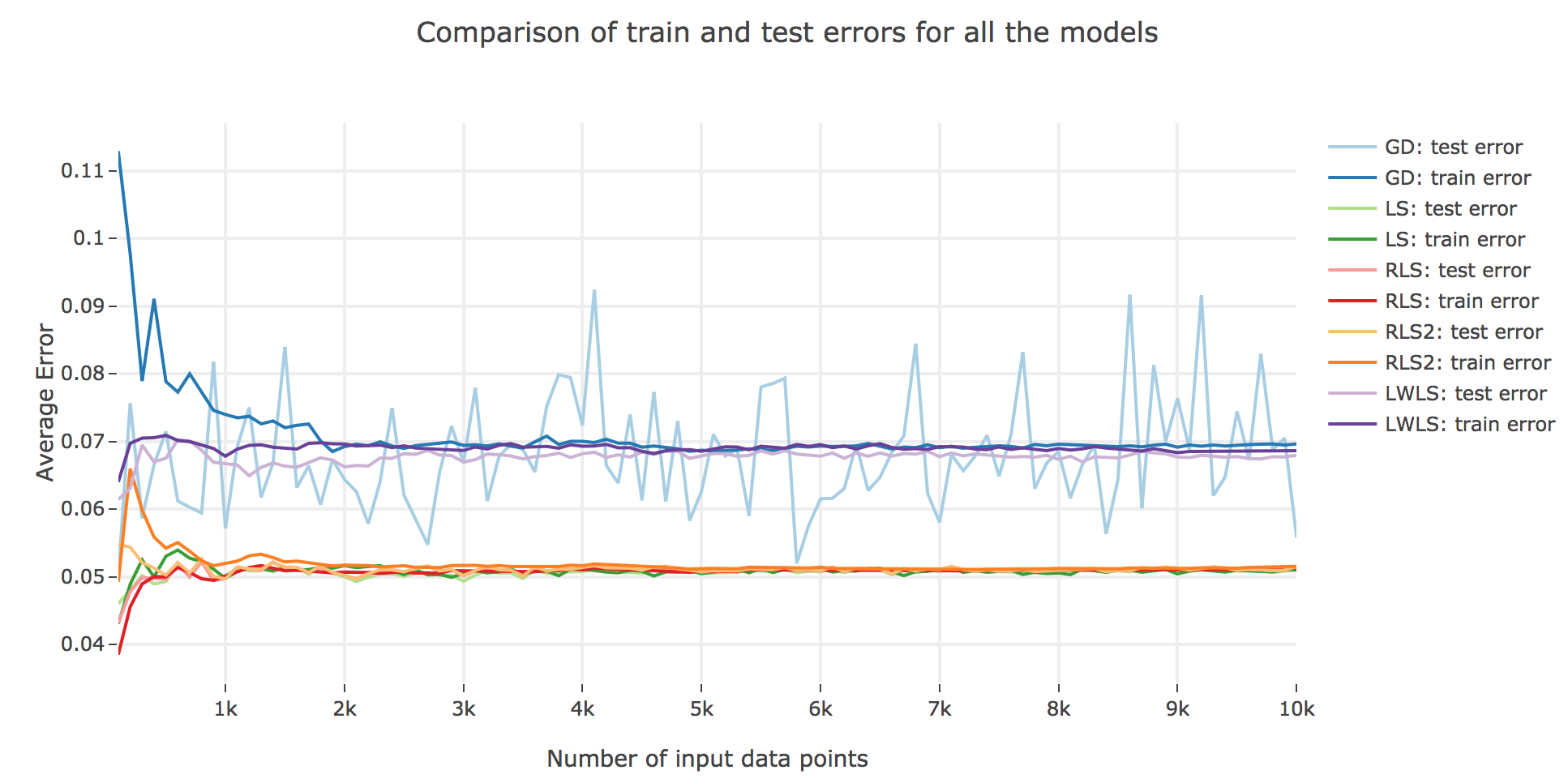
The obtained LWLS errors are rather similar to the ones of the Gradient Descent (GD) method. Basically, the models we reviewed are twofold, with respect to their train/test errors:
-
the ones that perform the most poorly are GD and LWLS, with an average error around $0.07$. It should be noted, though, that the GD test error is very unstable compared to the LWLS error, which is almost monotonous
-
the models with the highest accuracy (i.e. the lowest errors) are the LS, RLS, and RLS with Sherman-Morrison (RLS2) ones: these are all least-squares-related algorithms, the only difference between them being the updating mechanism: the batch LS computes the best estimator in one go, whereas RLS and RLS2 proceed incrementally. Their errors slightly differ for a few ($≤ 1000$) number of input data points:
- the LS and RLS methods have really similar errors (RLS being slighly better)
- but the RLS2 train error is a little bit higher than the other two: this can be accounted for by the fact that the pseudo-inverse calculation resulting from the Sherman-Morrison lemma is too rough at first (it has had time to sufficiently converge toward the actual pseudo-inverse with so few iterations)
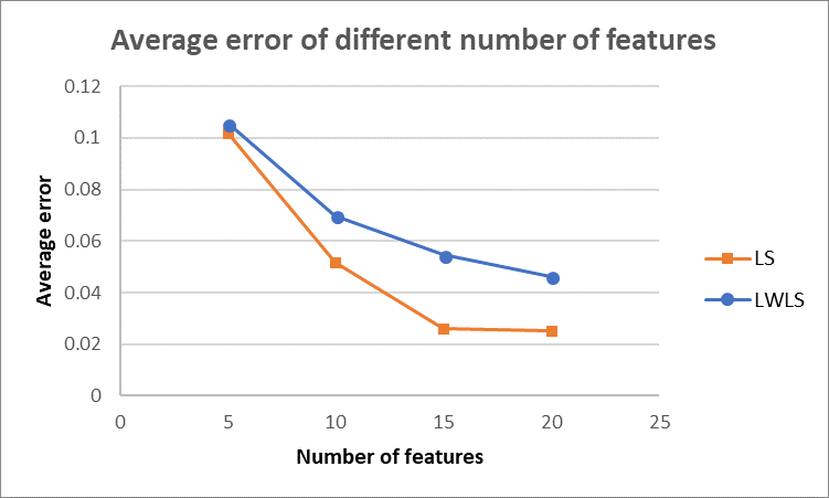
As for the average error depending on the number of features, we made the following plot by averaging over $10$ trials. As shown in the figure below, the average error decreases for both LS and LWLS. And LS generates lower error for all the numbers of features than LWLS. However, as discussed in Q1.1, we should be careful with the possible overfitting issue, as the number of features goes up. Thus, an appropriate number of features should be selected by considering both average error and overfitting problems.
Depending on the circumstances, how would you choose between an incremental method and a batch one?
Incremental methods seem to be more fitted for online learning situations: when
- there is a input stream of data points, processed one after another over time (so that we don’t have the full training set at once)
- we want the algorithm to be as fast as possible
- we don’t care too much about the accuracy (compared to the accuracy we could reach with batch methods)
We have encountered a similar situation in computational neuroscience courses, with the Rescola-Wagner rule (also known as the delta-rule).
On the other hand, batch methods come in handy when we
- have all the training set at hand
- don’t care that much about the algorithm taking a little more time
- want the supervized-learning algorithm to be as accurate as possible (i.e. we want the best unbiaised estimator for the training set at hand)
What modifications (other than modifying the meta-parameters) could you bring to the algorithms to get even more accurate approximations?
We could
-
try to vary the “types” of kernels used to approximate the ouput: instead of just settling for Gaussian kernels, we could use a combination of other kernels as well: sinc, triangle, Laplace, Cauchy, etc…
-
use several epochs for the incremental methods: that is, instead of just going through the training set once, we could repeat the training several times over the input data points, which would result in the training error decreasing more and more. But we would have to be careful not to overfit the training data (as a result of too many epochs)!
-
go as far as to develop a hybrid model to strike a better balance between speed of execution/online learning and accuracy: for instance, we could incrementally use batch methods over mini-batches (of given fixed size), one after the other, and then combine the models learnt on each mini-batch with a “voting” mechanism to choose the predicted output. The size of the mini-batches would then be chosen to meet a compromise between online flexibility/speed (smaller mini-batches) and accuracy (larger mini-batches).
Leave a comment