Exercise 1: softmax Gibbs-policy
Exercise 1: softmax Gibbs-policy
Younesse Kaddar
Static action choice and rewards
We assume that there are two types of flowers:
- blue flowers (which we give the index 1)
- yellow flowers (with index 2)
The flowers carry nectar rewards $r_1$ and $r_2$, and we assume that the bee’s internal estimates for the rewards are $m_1$ and $m_2$. The bee chooses the flowers according to a softmax-policy based on its internal reward estimates,
\[p(c=i) = \frac{\exp(β m_i)}{\exp(β m_1) + \exp(β m_2)} \quad \text{ for } i=1, 2\]a). Show that $\sum\limits_{ c=1 }^2 p(c)=1$
It’s a straight-forward calculation:
\[\begin{align*} \sum\limits_{ c=1 }^2 p(c) & = \frac{\exp(β m_1)}{\exp(β m_1) + \exp(β m_2)} + \frac{\exp(β m_2)}{\exp(β m_1) + \exp(β m_2)} \\ & = \frac{\exp(β m_1) + \exp(β m_2)}{\exp(β m_1) + \exp(β m_2)} = 1 \end{align*}\]b). Show that you can rewrite $p(c=1)$ as $p(c=1) = \frac{1}{1 + \exp(β (m_2-m_1))}$
By divinding the numerator and the denomator of $p(c=1) = \frac{\exp(β m_1)}{\exp(β m_1) + \exp(β m_2)}$ by $\exp(β m_1) ≠ 0$ (which amounts to multiplying both by $\exp(-β m_1)$), the result follows immediately (under the hood, we also use the fact that $\exp$ is a group homomorphism between $(ℝ,+)$ and $(ℝ^\ast_+,×)$).
Thus:
$p(c=i)$ is a sigmoid of $(m_i - m_{1-i})$
c). Plot the formula in b) as a function of the reward difference $d = m_2 - m_1$. Choose $β=1$ and choose the range of differences $d$ yourself.
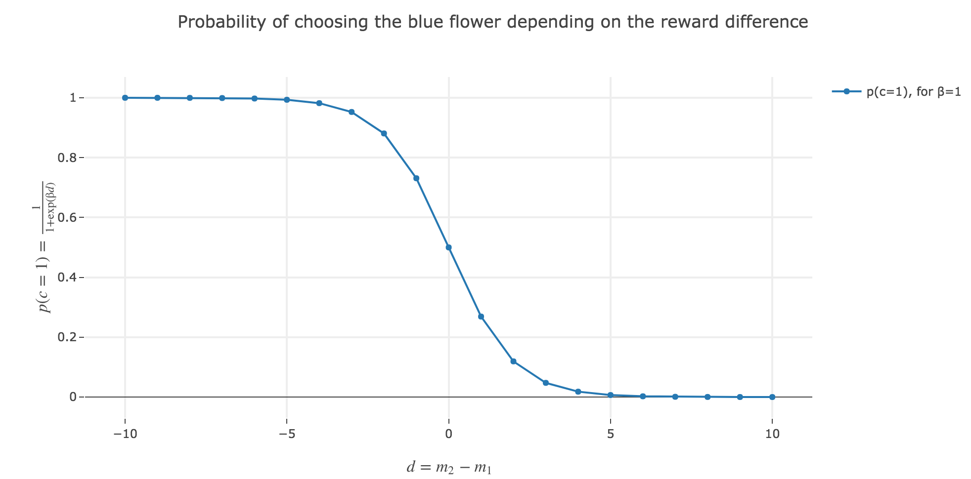
What happens if $d$ gets very large? What happens if $d$ is very small (= negative)?
As $p(c=1)$ is a sigmoid of $-d$:
- \[p(c=1) \xrightarrow[d \to +∞]{} 0\]
- \[p(c=1) \xrightarrow[d \to -∞]{} 1\]
What does that say about the bee’s choice?
The larger the reward difference $d ≝ m_2 - m_1$, the better the bee estimates the yellow flower (number 2) compared to the blue (first) one. As a result, the lower the probability $p(c=1)$ of the bee landing on the blue one.
Analogously, the lower the reward difference, the worse the yellow flower (from the bee’s point of vue), and the greater the probability $p(c=1)$ of the bee landing on the blue flower.
And in between, the bee’s behavior is a mix between exploiting the most nutritious flower (according to the bee) and exploring the other one (which is what is expected).
d). Investigate the meaning of the parameter $β$.
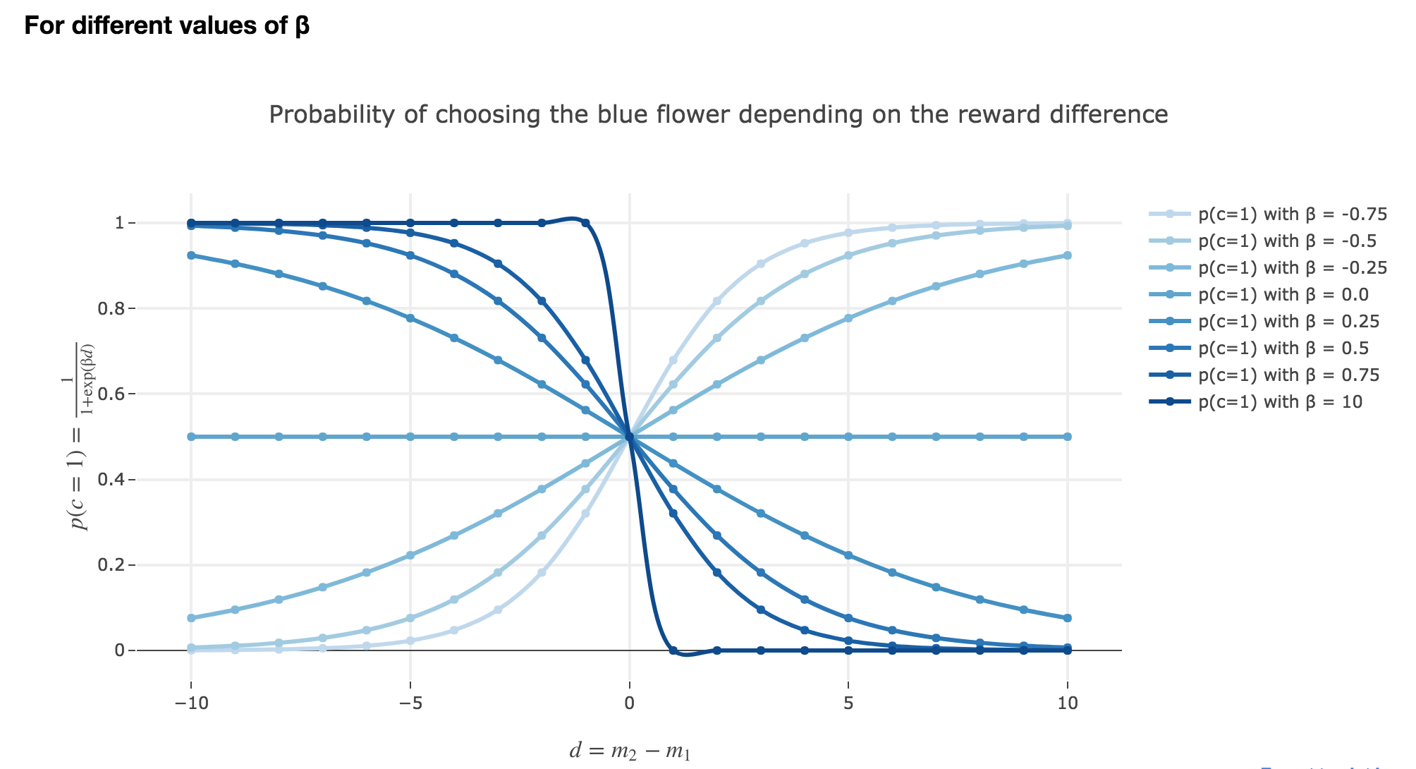
How does $β$ influence the exploitation-exploration tradeoff? What happens if you increase $β$ and make it very large, e.g $β = 10$? What happens if you let it go to zero?
The parameter $β$ plays a role analogous to the inverse temperature $β ≝ \frac{1}{k_B T}$ in statistical physics. That is, for $β ≥ 0$:
-
For $β ⟶ +∞$: the bigger the parameter $β$ (corresponding, in physics, to a low temperature/entropy), the more the bee tends to exploit the seemingly most nutritious flower. As a result:
- when $d > 0$ (i.e. the yellow is avantageous), the probability of the bee landing on the blue flower rapidly decreases to $0$
- when $d < 0$ (i.e. the blue flower is more advantageous), the probability of the bee landing on the blue flower rapidly increases to $1$
-
For $β ⟶ 0$: the lower the parameter $β$ (high temperature/entropy in physics), the more the bee tends to explore the flowers. Indeed:
- as $β ⟶ 0$, $p(c=1)$ becomes less and less steep, to such a point that it ends up being the constant function $1/2$ when $β=0$ (at this point, the bee does nothing but exploring, since landing on either of the flowers is equiprobable, no matter how nutritious the bee deems the flowers to be)
What happens if it becomes negative? Do negative $β$ make any sense?
As
\[p(-β, d) = \frac{1}{1 + \exp(-β d)} = \frac{1}{1 + \exp(β (-d))} = p(β, -d)\]The graphs for $-β < 0$ are symmetric to those for $β > 0$ with respect to the y-axis, which makes no sense from a behavioral point of vue: it means that: the most nutritious a flower appears to the bee, the less likely the bee is to land on it (and conversely)!
e). Imagine that there are $N$ flowers instead of just two. How can you extend the above action choice strategy to $N$ flowers?
To continue drawing a comparison with statistical physics: in physics, the probability that a system occupies a microstate $s$ is given by
\[p(s) = \frac {1}{Z} \exp(-\beta \underbrace{E_s}_{\rlap{\text{microstate energy}}})\]Where the partition function $Z ≝ \sum\limits_{ s’ } \exp(-β E_{s’})$ is a normalization constant.
Likewise, here, the natural generalization is given by:
\[p(c) = \text{Const} × \exp(β m_c)\]where the normalization constant $\text{Const}$ is equal to
\[\text{Const} = \sum\limits_{ c' } \exp(β m_{c'})\]so that the probabilities add to $1$.
Therefore, overall, the action choice strategy can be extended to $N$ flowers as follows:
\[∀ c ∈ \lbrace 1, ⋯, N \rbrace, \quad p(c) ≝ \frac{\exp(β m_c)}{\sum\limits_{ c' = 1}^N \exp(β m_{c'})}\]
How can you trade off exploration and exploitation for the $N$-flower case ?
As before (which was a particular case with $N=2$), the exploration-exploitation tradeoff depends on the value of $β$:
-
the bigger the parameter $β$, the more the bee exploits the flower it currently considers as the most nutritious
-
the lower the parameter $β$, the more the bee explores all the flowers
f). Imagine that there are $N$ flowers, yet the rewards on these flowers, $r_c(t)$ change as a function of time. How should the bee adapt its internal estimates $m_c(t)$?
When the time is discrete: we have seen, in class, three ways for the bee to update its internal estimates:
-
The greedy update:
\[m_c ≝ \underbrace{r_{c,i}}_{\text{lastest reward received from this flower}}\] -
The batch update: for $M ∈ ℕ^\ast$:
\[m_c = \frac 1 {M} \sum\limits_{ i=1 }^M r_{c,i}\] -
The online update/the delta-rule: for a learning rate $ε > 0$:
\[m_c \overset{\text{is updated as}}{⟶} m_c + ε (r_{c,i} - m_c)\]
If the time is now continuous:
By denoting by $T_c(t)$ the time that elapsed, at time $t$, since the last time (strictly before $t$) the bee visited the flower $c ∈ \lbrace 1, ⋯, N\rbrace$, the analogous continuous-time updates are:
-
The greedy update:
\[m_c ≝ r_c(t)\] -
The batch update: for $M ∈ ℕ^\ast$, and if
- $t_0 = 0$
- $t_{n+1} = T_c(t-t_n)$
- $\sum\limits_{ i=0 }^M t_i = t$
-
The online update/the delta-rule: for a learning rate $ε > 0$:
\[m_c(t) = m_c(t-T_c(t)) + ε \Big(r_c(t) - m_c(t-T_c(t))\Big)\]
e). Given the learning rules you developed in f), what will happen to the bee’s internal estimates $m_c(t)$, if the rewards stay constant for all $c$?
When it comes to the batch and greedy updates: if the rewards stay constant, so do the internal estimates, as soon as the bee lands on the corresponding flower.
The situation is trickier for the online update (so we will focus on this update from now on).
As we have seen in class:
\[m_c(t) \xrightarrow[ t \to +∞]{} r_c\]How does that depends on the parameter $β$?
As the update of $m_c$ is done whenever the flower $c$ is visited by the bee:
-
If $β$ is big (exploitation mode): the most nutritious a flower $c$ seems to the bee, the more often the bee will visit it, and the faster the convergence of $m_c(t)$ toward $r_c$
-
If $β$ is low (exploration mode): the convergence speed is as independent of the appeal of a flower $c$ as $β$ is low, since the lower the parameter $β$, the more often the bee explores (leading to the update of the explored flowers).
What is the characteristic time constant of convergence for the learning rules, i.e. how fast do the estimates converge to their real values?
For the sake of convenience, let’s assume $T_c(t) = T_c$ is constant. We have
\[m_c(t) = (1-ε) \, m_c(t - T_c) + ε r_c\]As a result, if $t ≝ n \, T_c$:
\[m_c(t) = (1-ε)^n \Big(m_c(0) - r_c\Big) = (1-ε)^{t/T_c} \Big(m_c(0) - r_c\Big)\]So for $t = τ$ the characteristic time constant, we have, as in physics:
\[\frac 1 {\mathrm{e}} \Big(m_c(0) - r_c\Big) = m_c(τ) = (1-ε)^{τ/T_c} \Big(m_c(0) - r_c\Big)\]And finally:
\[\begin{align*} & \quad \frac 1 {\mathrm{e}} = (1-ε)^{τ/T_c} \\ ⟹ & \quad τ = - \frac{T_c}{\ln(1-ε)} \\ \end{align*}\]Therefore:
Assuming that $T_c(t) = T_c$ is constant for the flower $c$, the characteristic time constant of convergence for the online update rule is equal to
\[τ ≝ - \frac{T_c}{\ln(1-ε)}\]
Leave a comment